Classification

Classification (or categorization) is a task where inputs are compared to possible categories and assigned to the most likely one.

2D binary classification

The goal is to find a line or curve, called a decision boundary, that separates the two classes.

Example:

• we have eggs and we suppose we can tell whether one is fertilized or not by measuring its weight and length
• we determine manually the "true" status of some eggs using candling (shining light through the egg)
• this human-labeled data (weight, length, and fertilization status) is given to the computer
• the computer learns to predict fertilization status based on the features (weight and length)
• once trained, the model can classify new eggs without known labels:
  • eggs on the red side → fertilized
  • eggs on the blue side → unfertilized

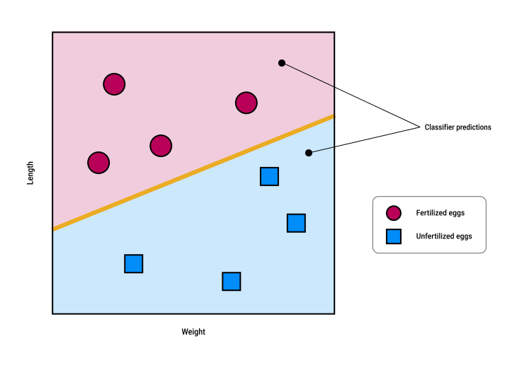
In more complex cases, decision boundaries may be curved or fuzzy:

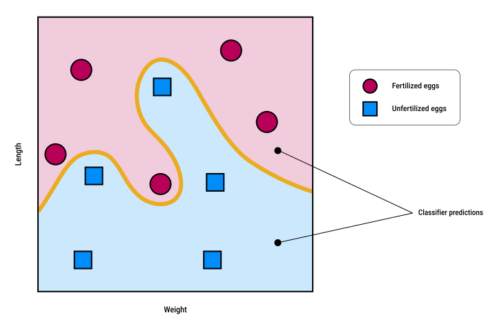
Each region of the plot represents a decision region, and the dividing lines or curves are the decision boundaries.

When classes overlap, no perfect boundary exists:

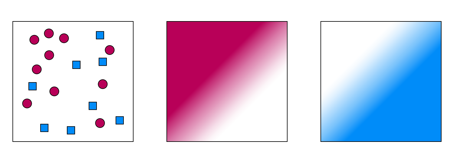
• instead, the classifier assigns a probability to each class
• points in the dark-red region are probably fertilized
• points in the dark-blue region are probably unfertilized
• points in lighter areas are uncertain

The final decision depends on our policy or which kinds of mistakes we are willing to accept:

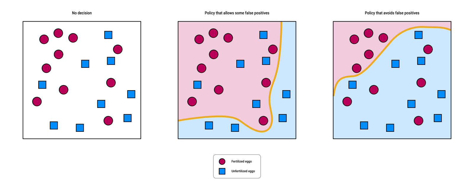
• with a policy that allows some false positives:
  • some unfertilized eggs are labeled as fertilized
  • this may waste time and resources, since unfertilized eggs will not hatch
• with a policy that avoids false positives:
  • some fertilized eggs are labeled as unfertilized
  • this risks losing potential chicks, which are more valuable

Classification decisions are guided by:

• model probabilities
• evaluation metrics (such as accuracy, precision, and recall)
• human judgment
• real-world considerations

2D multiclass classification

Assigning one of several possible classes to an input is called multiclass classification.

Example:

• the task is now to classify eggs into three categories:
  1. winners – viable fertilized eggs, sellable
  2. yolkers – unfertilized but safe to eat
  3. quitters – fertilized but unsafe, to be discarded
• we still suppose we can classify them just on the basis of their weight and length

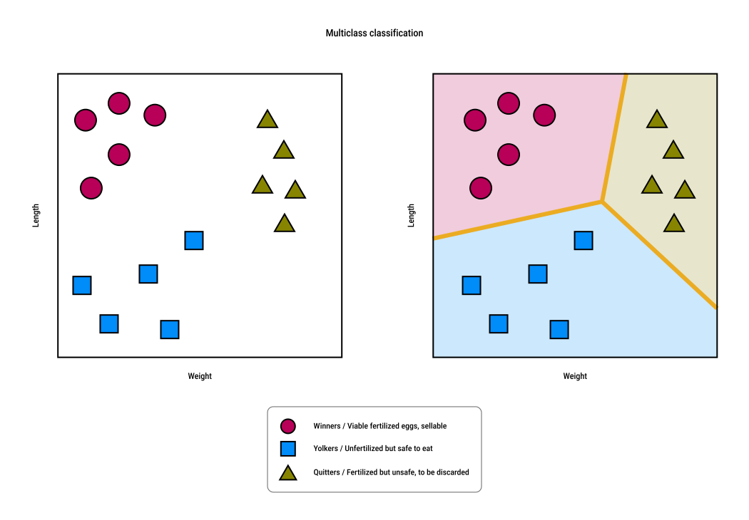
Each class forms a group, and decision boundaries separate the different groups.

New data is classified based on which group it falls into.

Multiclass classification

Multiclass problems can be solved by combining multiple binary classifiers, which are simpler and faster.

There are two popular methods.

One-Versus-Rest (OvR)

One-Versus-Rest (OvR) (or Binary Relevance) creates one binary classifier per class, where each classifier separates that class from all the other classes combined.

For example, with five classes (A–E):

• instead of building one complicated classifier, we build five separate binary classifiers
• classifier A distinguishes A vs. not A
• classifier B distinguishes B vs. not B, and so on

Each classifier:

• learns its own decision boundary separating one class from all others
• produces a probability that a sample belongs to its class.

To classify a new sample, we run it through all classifiers and assign it to the class with the highest probability.

Pros:

• simple and intuitive
• fast, especially if classifiers run in parallel

Cons:

• computational cost increases with the number of classes

One-Versus-One (OvO)

One-Versus-One (OvO) creates a separate binary classifier for every possible pair of classes.

For example, with four classes (A–D), we need six classifiers (A vs B, A vs C, A vs D, B vs C, B vs D, C vs D):

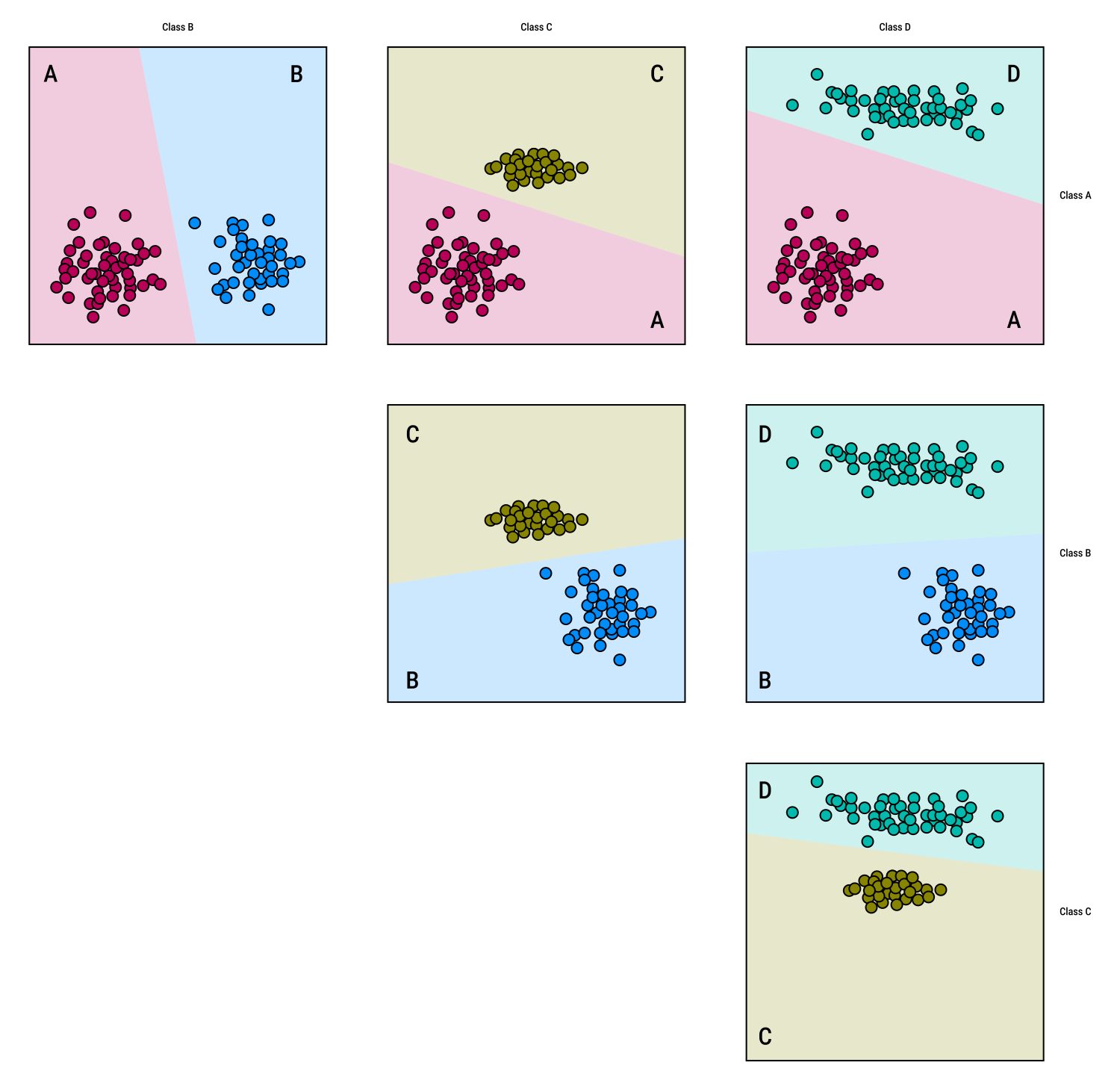
When classifying a new sample, we run it through all pairwise classifiers, and each one casts a vote.

The class with the most votes becomes the final prediction.

Pros:

• can be more explainable than other methods because each decision is traceable to specific class pairs
• helpful when classes overlap or boundaries are messy

Cons:

• requires far more classifiers than OvR, growing rapidly with the number of classes:
  • 4 classes → 6 classifiers
  • 20 classes → 190 classifiers
  • 30 classes → 435 classifiers
• training and evaluating all classifiers is computationally expensive
• beyond a certain number of classes, a single multiclass model becomes more efficient

Clustering (for unsupervised learning)

The general idea is to group the training set data into clusters, or similar chunks.

If the data has associated labels (supervised learning):

• suppose there are five different labels shown by color
• clusters can be formed by drawing a curve around each set of points
• extending those curves outward until they intersect covers the entire plane

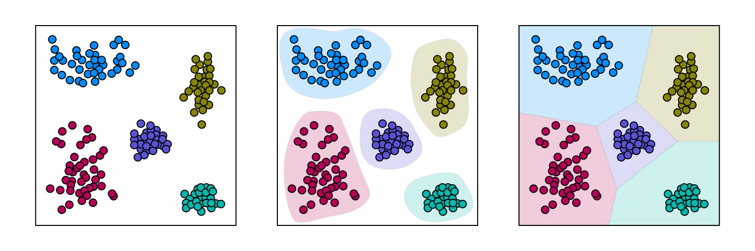
If the data has no associated labels (unsupervised learning):

• an algorithm must be told how many clusters (or regions) to find
• this "number of clusters" is represented with the arbitrary letter k
• k is a hyperparameter (a value chosen before training the system)
• the algorithm uses the geometric means of groups of points, so it is called k-means clustering

The freedom to choose the value of k can be both helpful and challenging:

• upside: if the number of clusters is known in advance, specifying k produces the desired result
• downside: if k is unknown, selecting too few clusters may combine distinct groups, while selecting too many may cause similar pieces of data to end up in different classes

For simple, low-dimensional data, the best k can be easy to see (k=5 gives the best result):

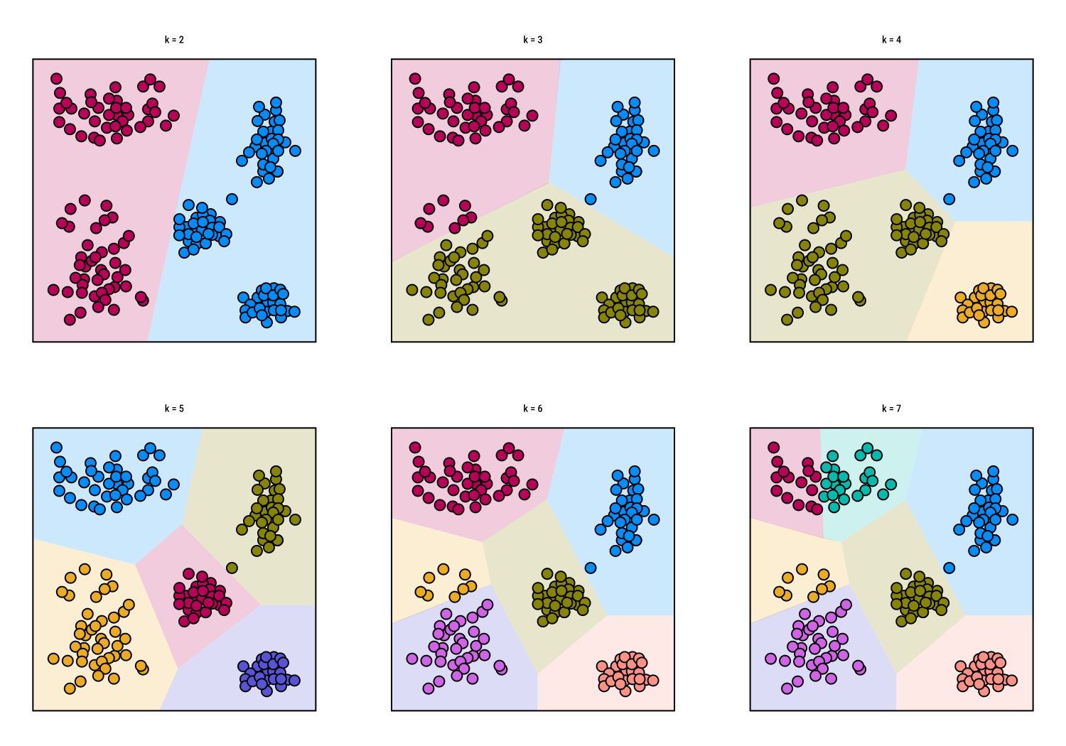
For higher-dimensional or complex data, identifying the optimal k in advance is difficult.

All is not lost:

• clustering models can be trained multiple times with different values of k (hyperparameter tuning)
• the downside is that this takes computational resources and time
• this is why it's so useful to preview the data with some kind of visualization tool prior to clustering
  • doing so can help pick the best value of k right away, or even identify a range of likely values
  • time and effort are saved by avoiding poor choices of k

Dimensionality and density

In theory, adding more features (dimensions) to data should help classifiers perform better by giving them more information.

However, beyond a certain point, adding more features actually harms performance.

This effect is known as the curse of dimensionality.

As data gains more dimensions, it becomes harder for a model to find meaningful patterns or decision boundaries.

The curse of dimensionality

To learn a good decision boundary, a classifier needs a dense set of training samples.

With few data points, it's easy to draw many different boundaries that separate them, making it hard to choose one that generalizes well:

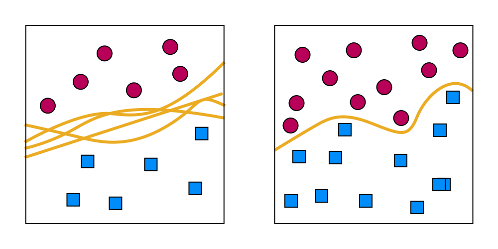
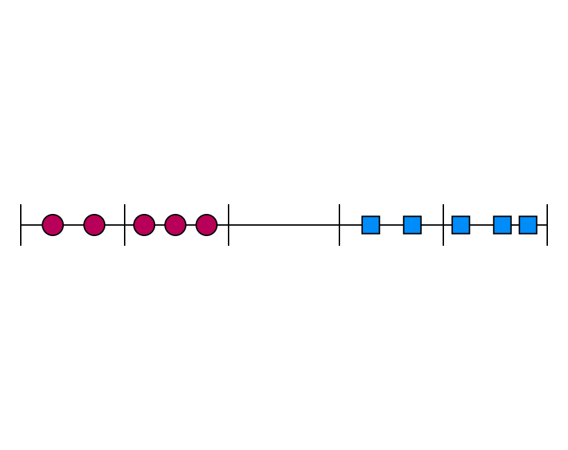
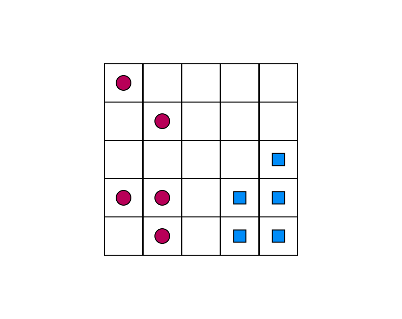
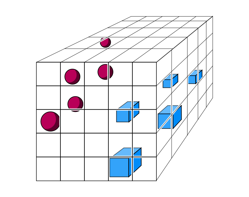
Using a dataset of 10 eggs with features scaled between 0 and 1, we see that as we add more features, the density decreases exponentially:

Dimensions	Explanation	Image
1D	With only one feature (e.g., weight) the data fits on a line from 0 to 1 dividing this line into 5 bins gives a density of 10 samples / 5 bins = 2 samples per bin on average this is enough to learn a reasonable boundary
2D	With two features (e.g., weight and length) the data fits a 2D square with 25 bins (5 × 5) with still only 10 samples, density drops to 10 / (5 x 5) = 0.4 most bins are empty, allowing many possible boundaries
3D	With three (e.g., weight, length, and volume) the data fits a 3D cube with 125 bins (5 × 5 × 5) with still only 10 samples, density drops to 10 / (5 x 5 x 5) = 0.08 almost all bins are empty, leaving insufficient data to reliably learn boundaries

As the number of features (dimensions) increases while the number of samples stays fixed, the data becomes sparse. This is the curse of dimensionality.

The problem isn't that it's hard to separate the data, but that it's too easy: many different boundaries fit equally well, but most will perform poorly on unseen data.

The blessing of non-uniformity and the manifold hypothesis

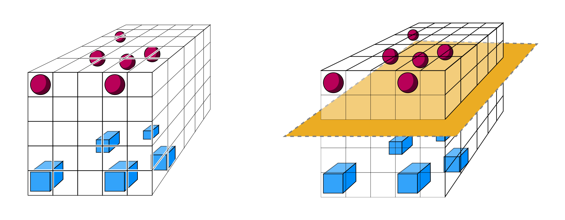
What mitigates this issue is the blessing of non-uniformity (or blessing of structure):

• in practice, both training and future data tend to concentrate in certain regions
• these regions have high local density, while most of the space remains empty
• these regions often lie on a lower-dimensional structure within the high-dimensional space
  • a manifold is a precise mathematical way to describe such a structure
  • it is a lower-dimensional space embedded in a higher-dimensional one
  • e.g., a 2D surface (like a sheet of paper) embedded in 3D space is a 2D manifold
• classifiers can focus on these manifolds
• when classes are well-structured and separated along these manifolds, many different boundaries can generalize well, even in very high-dimensional spaces

Both the curse and blessing are empirical observations, and not hard facts we can always rely on.

In general, we can mitigate the curse of dimensionality by:

1. collecting more data (more data increases density in the important regions)
2. reducing the number of features (dimensionality reduction)

The curse of dimensionality is one reason why machine learning systems often need huge amounts of data for accurate learning.

High-dimensional weirdness

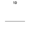
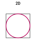
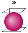
Imagine a sphere perfectly fitting inside a cube. How much of the cube's volume does it occupy?

Dimensions	Explanation	Image
1D	the cube is just a line segment, and the sphere is also a line segment that exactly matches so the sphere fills 100% of the cube
2D	the cube becomes a square and the sphere becomes a circle that touches the midpoint of each side area of the circle divided by area of the square ≈ 0.8 circle fills ≈ 80% of the square
3D	the cube is a regular cube and the sphere fits inside it, touching the center of each face volume of the sphere divided by volume of the cube ≈ 0.5 sphere fills ≈ 50% of the cube

As dimensions increase, the ratio keeps shrinking.

In higher dimensions, the volume of the largest hypersphere inside a hypercube drops rapidly. By the 10th dimension, the hypersphere occupies almost none of the hypercube's volume:

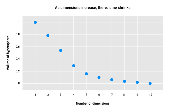
This is surprising, but mathematically correct.

High-dimensional geometry behaves in strange, unintuitive ways.

When working with multidimensional data, we cannot rely on intuition but must use precise mathematical reasoning.