Reinforcement learning

Reinforcement learning (RL) is a way to train machine learning systems without labels.

Instead of being told the correct answer:

• the system learns by trying different actions and seeing which ones lead to better results
• progress toward a goal is rewarded, helping the system gradually learn what works best

RL encompasses many algorithms and is an active research area.

Basic ideas

In reinforcement learning, a decision-maker called an agent interacts repeatedly with an environment.

The agent takes actions that affect an environment and receives feedback, called a reward.

By trying different actions and learning from rewards over time, the agent gradually improves its decisions through trial and error.

RL is especially useful when the best action isn't obvious or consistent. It can handle uncertainty and varying conditions, learning strategies that perform well even in unpredictable environments.

Basic structure of reinforcement learning

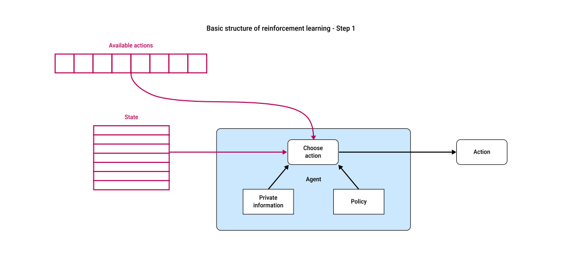
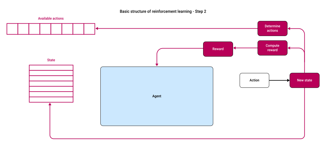
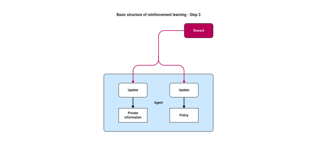
Reinforcement learning can be understood as a three-step cycle between an agent and its environment.

RL begins by placing the environment in an initial state (for example, the starting board in a game).

One complete cycle of training, from beginning to end, is called an episode (for example, a full game).

This three-step cycle repeats over many episodes:

Step	Explanation	Image
Step 1: agent selects an action	The environment provides: the current world state, described by state variables (a set of numbers): the complexity depends on the environment example: in a board game, the state includes positions of pieces, money, power-ups, etc. a set of possible actions the agent can take The agent: remains idle until the environment signals it's time to act chooses an action using a policy and private information such as what it's learned from previous episodes sends the chosen action to the environment (without directly performing it)
Step 2: environment responds	The environment: receives the action executes the action updates the state determines which actions are available to the agent in the new state (old actions are completely replaced) computes and sends the agent a reward (usually a single number) showing how good or bad its last action was based on goals defined by the system designer
Step 3: agent updates itself	The agent uses the reward to update its internal data and policy parameters. Rewards: helps the agent make better decisions if it encounters the same situation again may also influence the evaluation of earlier actions that led to the result

Big-picture considerations in RL

Agents may have:

• full observability: access to all state parameters
• partial observability: access to only some parameters
  • can save computation when some parameters are expensive to calculate
  • or simulate real-world situations (like hidden cards in poker)

When training agents with feedback, two big challenges come up:

1. credit assignment problem: when a final reward is received (win or loss), the agent must determine how much credit or blame to assign to intermediate actions that led to the outcome

2. explore-exploit dilemma: the agent must decide whether to exploit known actions it knows work, or explore new actions that might do better or worse

Understanding rewards

Rewards guide an agent to select actions that maximize performance.

All rewards received during an episode can be listed in order. Their sum is the total reward.

For any specific move in that list, the total future reward (TFR) equals:

• the reward for that move, plus all rewards that follow it
• e.g., the first move's TFR = total reward

TFR measures how much a move contributed in a specific episode.

However, TFR is not always reliable for predicting future outcomes because real environments are often stochastic (unpredictable):

• the same action in the same situation can produce different outcomes due to environmental changes
• e.g., a robot presses a remote power button: it works 100 times but fails on the 101st attempt if the battery is drained

To account for this uncertainty, we use a discount factor γ (gamma), between 0 and 1:

• represents our confidence that the environment will behave similarly in the future
• γ ≈ 1 → environment is deterministic → the same action likely yields the same reward
• γ ≈ 0 → environment is unpredictable → rewards may vary

Using γ, we modify TFR to obtain the discounted future reward (DFR):

• take the immediate reward (computed after the environment responds, so dependent on environmental changes and less reliable)
• discount later rewards by multiplying them by γ:
  • one step ahead → × γ
  • two steps ahead → × γ²
  • and so on

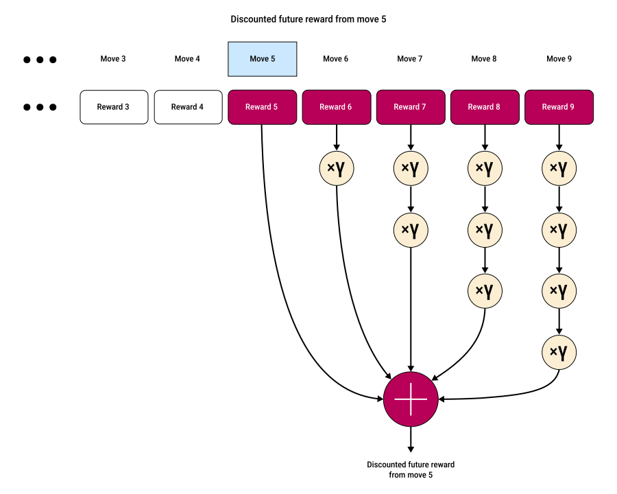
This reduces the weight of distant rewards, reflecting their increasing uncertainty.

Typical values of γ:

• often ≈ 0.8-0.9 initially
• then adjusted as we learn how predictable the environment actually is

Flippers

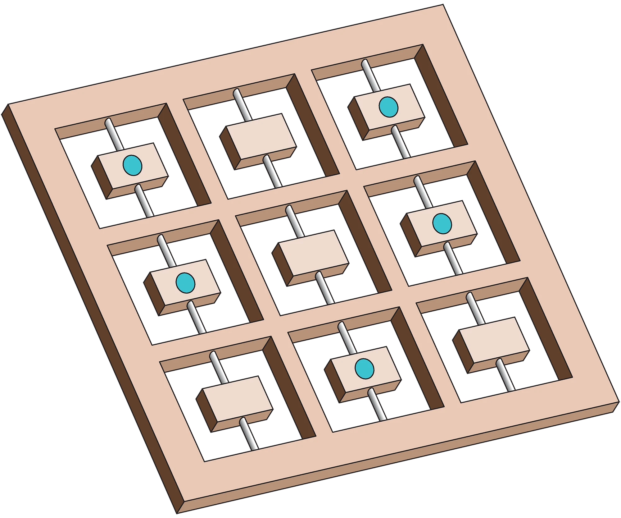
Flippers is a simple game used to explain reinforcement learning.

Concept	Explanation	Image
Game	3×3 grid of tiles each tile has two sides: blank or dot on each turn, the player flips one tile
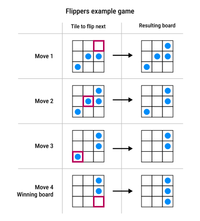
Goal	The goal is to get three dots in a row or column with all other tiles blank, using as few flips as possible.
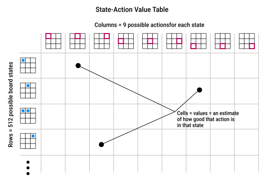
State-Action Value Table	The system can be represented as a table: rows = 512 possible board states columns = 9 possible actions for each state cells = values an estimate of how good a move is in that situation 512 rows × 9 columns = 4,608 values, all initially set to 0 because nothing has been learned yet
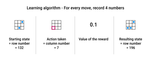
Transitions	During a game, the agent records all moves as "transitions" (bundles of 4 numbers): starting state action taken value of the immediate reward received resulting (or next) state These bundles are stored in a list that grows throughout the game.

L-learning

L-learning is a deliberately "lousy" (L) algorithm for learning to play Flippers created as a teaching step toward a better method.

Values

Only the winning move gets a reward that depends on the length of the game:

• winning in one move = highest reward (1)
• the reward decreases quickly as the number of moves increases

To estimate values:

• play a full game while recording all moves
• at the end of the game:
  • compute the Total Future Reward (TFR) for each action
  • since only the final move has a reward, all moves receive the same TFR equal to the final reward
  • moves are judged solely by whether they eventually lead to a fast win

Table update rule

The table entry for each move is replaced with that TFR:

• it overwrites old knowledge instead of refining it
• this is intentionally simple and won't perform very well

Over many games:

• the table gradually fills with learned TFR values
• the agent improves by selecting the highest-value action for each board state

Policy

To choose a move:

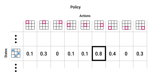
• for the current board state, choose the action with the highest value in that row
• if multiple actions tie, pick one at random
• in short: "Do the move that has worked best in the past for this situation"

Handling unpredictability

In the Flippers example, a random or unpredictable event can be represented by a "big truck" that occasionally shakes the board and randomly flips tiles, unexpectedly changing the game state.

The weakness of L-learning comes from its policy and update rule:

• the algorithm always selects the action with the highest value
• after each game, the TFR replaces the previous value in the table
• if a random event causes a normally good move to lead to a longer game, the lower reward overwrites the previous high value

As a result, a single unlucky event can erase knowledge of the best move. The algorithm "forgets" the best move and may make worse choices in future games.

Although random exploration may eventually rediscover the good move, this process can take a long time.

Q-learning

Q-learning is a "quality" (Q) algorithm that improves on L-learning:

• better computation and update of values
• a more effective action-selection policy

Q-learning is built around two ideas:

• it accounts for uncertainty from the start
• learning happens continuously: instead of waiting for a final outcome, the environment provides immediate rewards after each action

Values

Values are estimated as:

• the immediate reward
• plus the discounted future reward (γ × max value of next state)
  • γ (gamma) is the discount factor to account for uncertainty
  • value of next state:
    • are available in the recorded "bundle of 4 numbers" we've been using for L-learning
    • start as arbitrary initial values (often zero) and gradually become more accurate

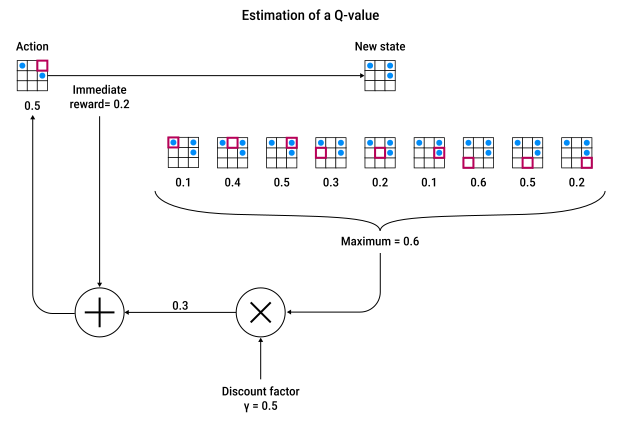
Table update rule

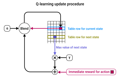
Rather than replacing a cell's value with each new estimate, Q-learning blends the old and new values using the learning rate (α, alpha):

• α = 0 → no change
• α = 1 → completely replace the old value
• in practice, α is set close to 1 (e.g., 0.9 or 0.99):
  • values near 1 cause new values to dominate but some past knowledge is retained
  • α = 0.9 → the updated value is 10% old value and 90% new value
  • the optimal α is found experimentally
• note: this "learning rate" is unrelated to the one used in backpropagation

Advantages over L-learning:

• incorporates both immediate and future rewards
• discounts uncertain future rewards
• smoothly updates values to handle randomness
• iteratively converges to accurate values through repeated updates

Policy

Q-learning policies aim to balance exploitation and exploration.

Common Q-learning policies:

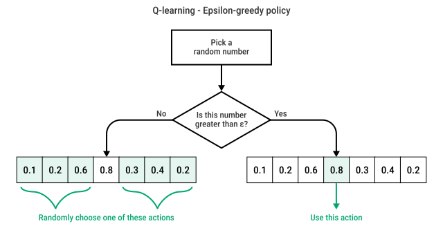
1. epsilon-greedy (or epsilon-soft) policy
   • choose a small number ε between 0 and 1 (typically close to 0.01)
   • each time an action is selected:
     • pick a number between 0 and 1 from a uniform distribution
     • if the number is greater than ε, choose the action with the highest value
     • if the number is less than ε, choose an action at random
   • this approach exploits the best-known action while occasionally exploring others
   • 
2. softmax policy
   • convert the values for a state into a probability distribution using a softmax function
   • select an action randomly according to these probabilities
   • actions with higher values are chosen more often, but all actions have a chance of being selected
   • the probability of choosing an action reflects its current value:
     • when values are updated, the action probabilities are updated immediately
     • higher values increase the chance of selection
     • lower values reduce the chance of selection
     • softmax keeps action selection aligned with the latest knowledge

Softmax can sometimes be too sensitive or introduce persistent randomness, which may prevent learning from stabilizing.

An alternative called mellowmax uses a different mathematical approach to encourage more stable learning while still allowing exploration.

The policy parameters, learning rate, and discount factor are typically chosen through trial and error, as their best values depend on the specific task and environment.

Learning from zero knowledge

Q-learning starts with a table initialized to zero.

At the start, the system behaves randomly because all values are the same, and it has no information to guide its choices.

Learning begins when rewards are encountered. Eventually, by chance, the system reaches a winning outcome (a "victory"), which produces a positive reward.

That reward updates the value of the action that led to the success.

Because the update rule looks one step ahead, rewards from winning outcomes gradually influence the earlier actions that led to them. This creates a ripple effect where earlier decisions gain value over time.

In this way, Q-learning learns which early decisions are good, even if the reward only appears at the end of the game.

Over time, exploration ensures that all actions are tried, and values increasingly reflect the true expected rewards of actions.

This process eventually stabilizes, a property known as convergence:

• Q-learning is mathematically proven to converge
• the speed of convergence depends on task complexity, environment unpredictability, and chosen parameters

Q-learning solves key reinforcement learning problems:

1. the credit assignment problem: rewards propagate "backward" through earlier actions
2. the exploration–exploitation dilemma: policies like epsilon-greedy or softmax balance exploration with exploitation

SARSA

Q-learning updates values as if the agent will always choose the highest-value action, even though the actual policy (like epsilon-greedy or softmax) may choose otherwise.

This mismatch can lead to inaccurate updates.

SARSA addresses this issue.

SARSA algorithm

SARSA bases its updates on the action that is actually taken next, rather than the best possible one.

SARSA is called an on-policy method because it learns the value of the policy it actually follows. By contrast, Q-learning is off-policy.

SARSA = State → Action → Reward → State → Action.

At each step (SARSA'):

• executes one action (the first A)
• selects and stores the next action (A') in advance using the policy
• updates values using that actual next action

Like Q-learning, SARSA is proven to converge, and in practice it often starts producing useful results faster.

Limitations of state-action value tables

These tables store all possible state-action values, which works for small problems but scales poorly:

• 4×4 board → 43 million states
• 5×5 board → 850 billion states
• Go (19×19 board) → unimaginably huge state space, making tables impractical

Deep reinforcement learning addresses this by replacing tables with neural networks:

• the table is treated as a function mapping states to action values
• neural networks approximate this function by taking the board state as input and predicting values for each possible action
• once trained, the agent chooses actions based on the network's predictions instead of storing massive tables

This approach enabled AlphaGo and AlphaZero to play Go at world-champion levels and has applications in video games, robotics, and healthcare.