Distance-Vector routing algorithm (DV)

The Distance-Vector (DV) algorithm allows each router to learn the best paths to destinations by exchanging information with its immediate neighbours.

It is:

• distributed:
  • every router participates in computing routes using only information from itself and its neighbours
  • there is no central routing authority that knows the complete network and calculates all paths
• iterative:
  • nodes repeat this process until nothing changes
  • the algorithm is self-terminating: no special "stop" message is needed
• asynchronous:
  • nodes do not have to wait for each other before acting

It is called distance-vector because each router maintains a vector of distances (costs) to all known destinations.

Bellman-Ford algorithm

Distance Vector (DV) routing is:

• an algorithm based on the Bellman–Ford shortest-path recurrence
• decentralized: it distributes the computation across routers

Each router only knows:

• the cost of its links to directly connected neighbours
• the distance vectors advertised by those neighbours (empty at the very beginning, populated through exchanges over time)

Bellman–Ford equation

To estimate the cheapest path from node \( x \) to node \( y \), node \( x \) checks all its neighbors \( v \) and chooses the route with the lowest total cost:

\[ D_x(y) = min_v\{ c(x, v) + D_v(y) \} \]

For each neighbor \( v \) of \( x \):

• \( c(x, v) \) = cost from \( x \) to direct neighbor \( v \)
• \( D_v(y) \) = neighbor \( v \)'s current estimated cost to \( y \)

In simple terms:

My best route to a destination is the cheapest route through any of my neighbours, based on the distances they currently advertise.

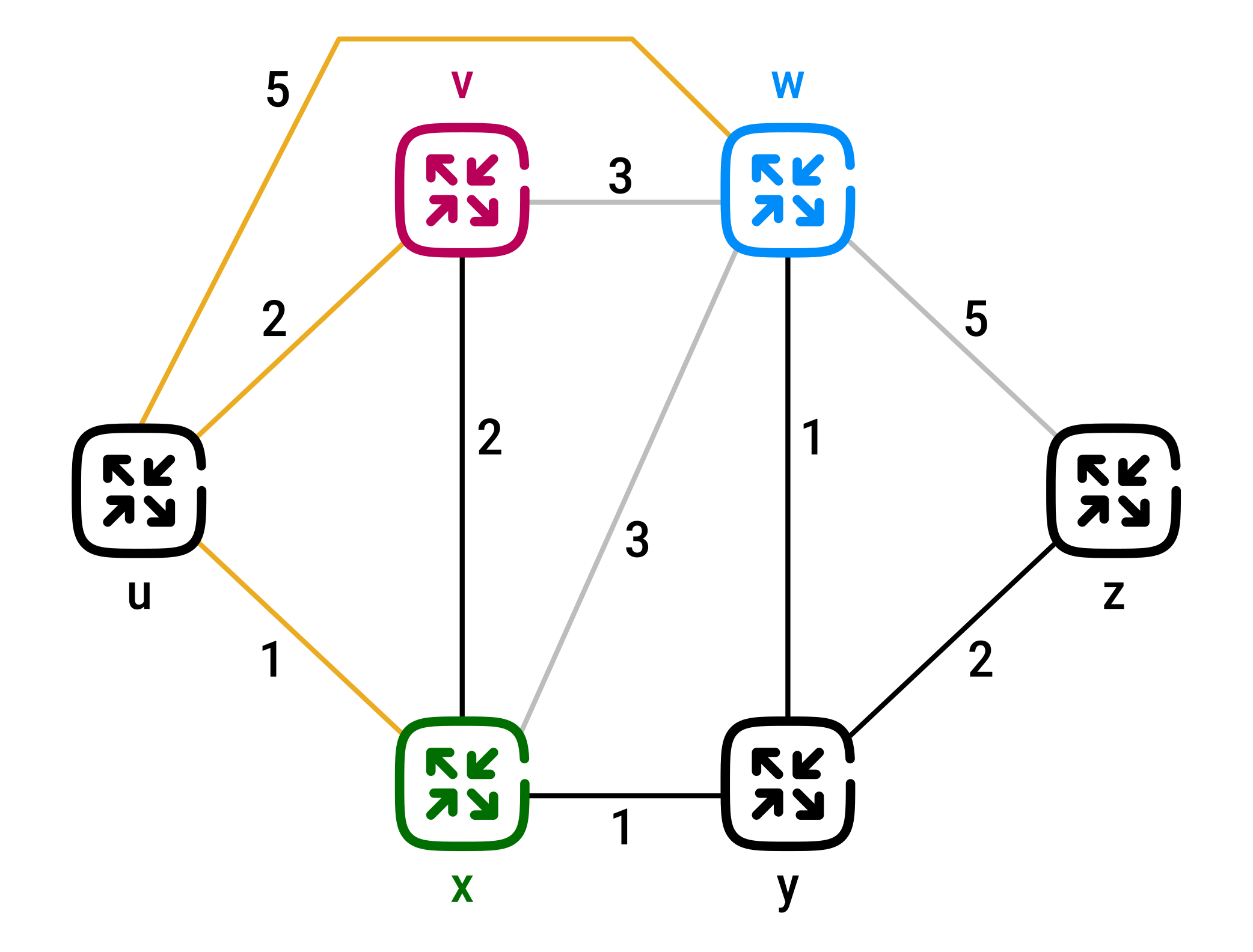
Suppose node \( u \) wants to estimate its cost to reach destination \( z \):

Neighbors of \( u \)	\( {\color{crimson}v} \)	\( {\color{ForestGreen}x} \)	\( {\color{navy}w} \)
Costs from \( u \) to neighbors	\( {\color{crimson}c(u, v) = 2} \)	\( {\color{ForestGreen}c(u, x) = 1} \)	\( {\color{navy}c(u, w) = 5} \)
Best known cost advertised from neighbors to reach \( z \)	\( {\color{crimson}D_v(z) = 5} \)	\( {\color{ForestGreen}D_x(z) = 3} \)	\( {\color{navy}D_w(z) = 3} \)
B-F equation	\[ \begin{aligned} D_u(z) &= min\{ {\color{crimson}c(u, v)+D_v(z)}, {\color{ForestGreen}c(u, x)+D_x(z)}, {\color{navy}c(u, w)+D_w(z)} \} \\ &= min\{ {\color{crimson}2+5}, {\color{ForestGreen}1+3}, {\color{navy}5+3} \} \\ &= min\{ {\color{crimson}7}, {\color{ForestGreen}4}, {\color{navy}8} \} \\ &= {\color{ForestGreen}4} \\ \end{aligned} \]
Result	The best next hop from \( u \) to \( z \) is \( {\color{ForestGreen}x} \)

DV algorithm

Each router uses the Bellman–Ford equation to maintain its distance vector and build its forwarding table.

A router maintains:

• a distance vector (DV), which estimates the cost to reach every destination in the network
• a next-hop entry indicating which neighbour should be used to reach each destination

Algorithm initialization at node \( x \):

for each destination y:
    if y == x:
        Dx(y) = 0
    else if y directly connected to x:
        Dx(y) = c(x,y)
    else:
        Dx(y) = ∞

for each neighbor v:
    send distance vector Dx to v

Algorithm main loop at node \( x \):

repeat forever:

    wait until:
        - a link cost c(x,v) changes, OR
        - a distance vector Dv is received from neighbor v

    for each destination y in N:
        Dx(y) = min over neighbors v { c(x,v) + Dv(y) }

    if Dx changed:
        send distance vector Dx to all neighbors

Convergence

Routers gradually improve their estimates by exchanging information with their neighbours.

Under stable network conditions, the estimated costs \( D_x(y) \) converge to the actual shortest-path costs \( d_x(y) \).

Once convergence occurs, each router knows the lowest-cost route to every reachable destination and can maintain a stable forwarding table.

If a link cost changes, routers exchange updated distance vectors and repeat the process until they converge again.

DV-style algorithms are used in real-world routing protocols such as RIP for IP networks, AODV for wireless networks, and DSDV for mobile networks.

Link-cost changes

When a link cost decreases

The link cost between x and y decreases from 4 to 1:

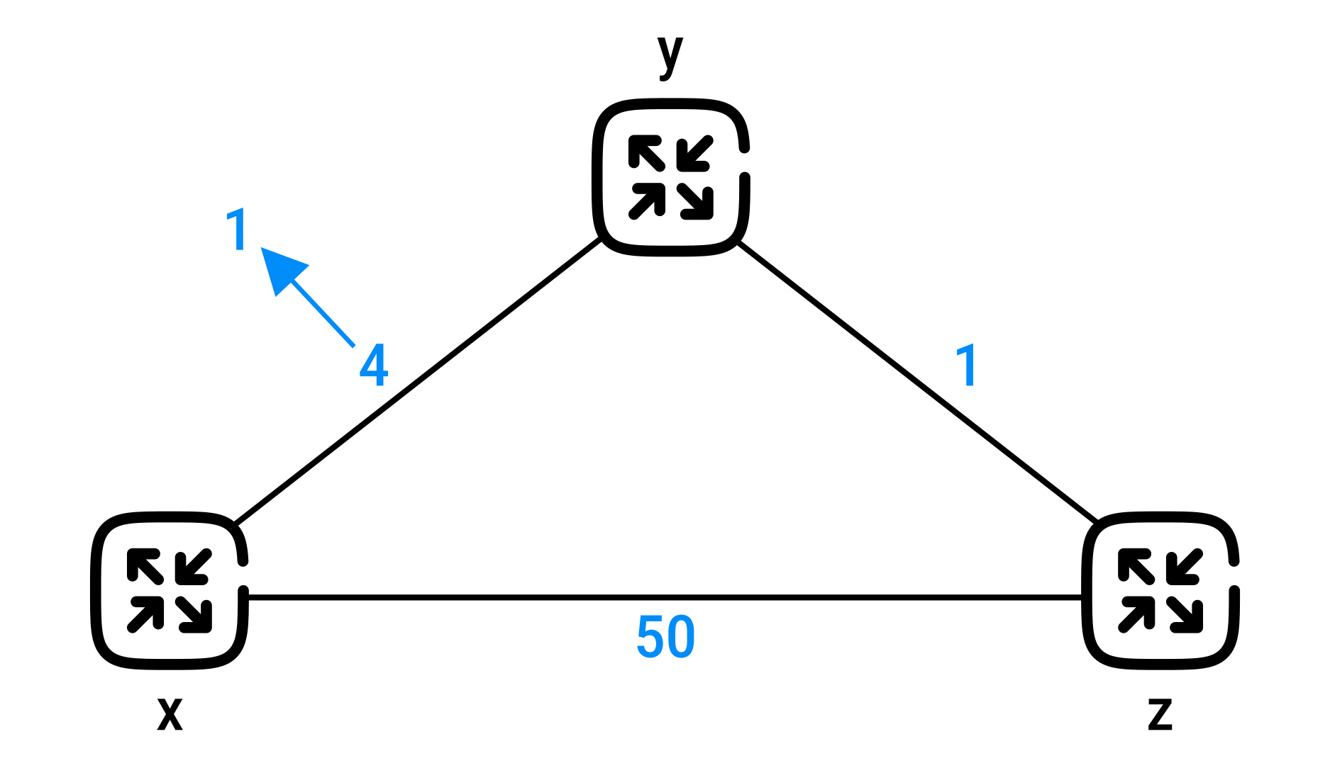
• y updates and advertises \( D_y(x) = 1 \ \) to its neighbors
• z thinks: "Great, then I can reach x via y for cost 2"
• z updates and advertises \( D_z(x) = 2 \ \) to its neighbors
• y receives the update, but its least-cost path is unchanged, so it sends no further updates

The network reaches a quiescent state after two iterations.

The decreased cost between x and y has propagated quickly: good news travels fast.

When a link cost increases

The link cost between x and y increases from 4 to 60:

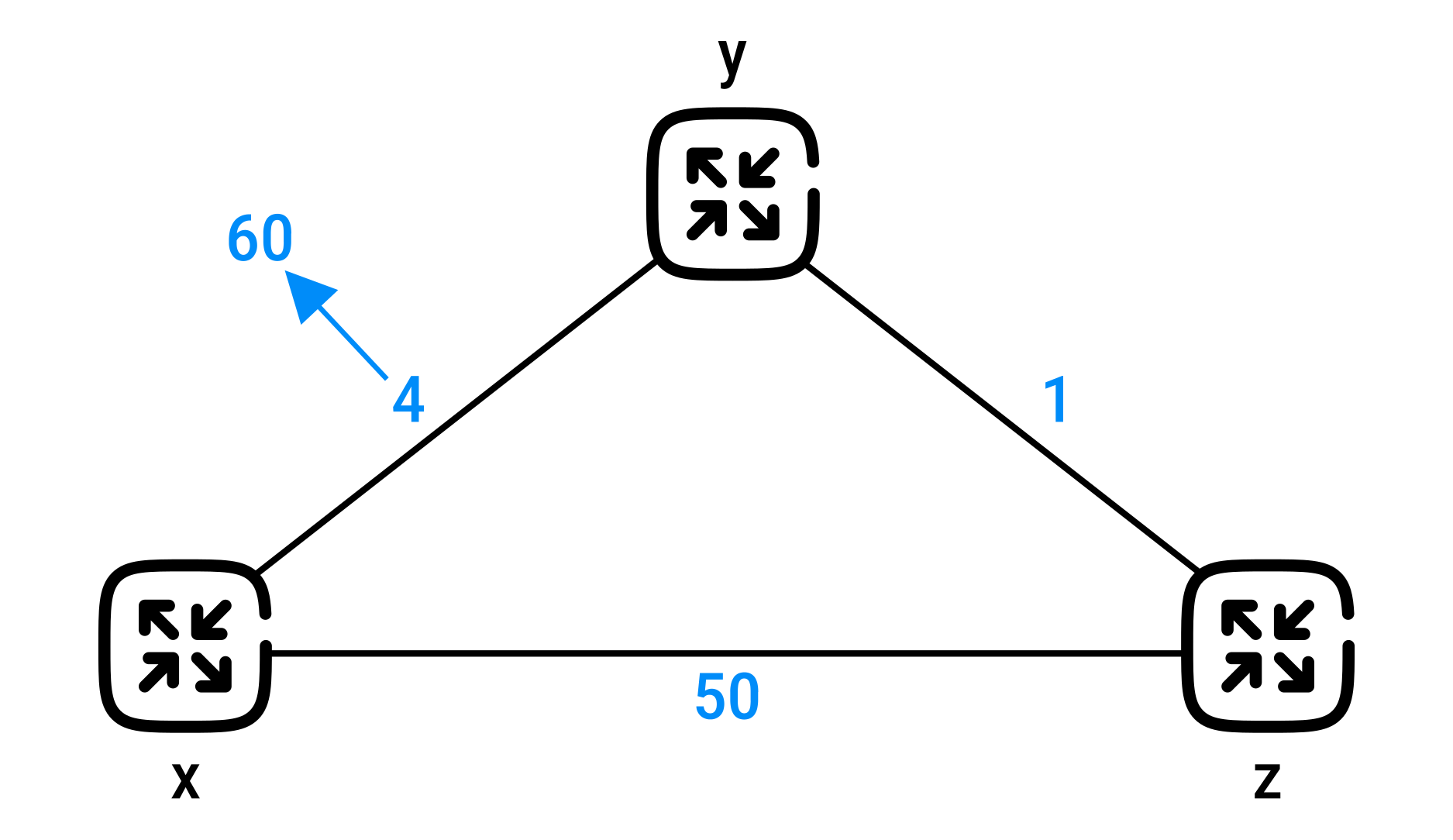
• y sees z advertising a cost to x of 5 and incorrectly updates \( D_y(x) = 1 + 5 = 6 \ \)
• y advertises the new cost, unaware that z's advertised cost of 5 was itself based on going through y
• z updates to 7 and advertises back
• each router believes the other router has a valid route to x, even though both routes ultimately depend on each other
• this creates a routing loop: y → z → y → z → …

The cost therefore increases one hop at a time:

6 → 7 → 8 → 9 → …

The process may take many iterations until the learned path cost exceeds the direct alternative (50), causing z to switch to the direct route to x.

The network reaches a quiescent state only after many iterations. The increased cost between x and y has propagated slowly.

This behavior is known as the count-to-infinity problem, which is why: bad news travels slow.

Poisoned reverse

This specific looping scenario can be avoided using the poisoned reverse technique.

Whenever a router reaches a destination through a neighbor, it advertises an infinite cost for that destination to that neighbor.

Example

Initially:

• y reaches x directly with cost 4
• z reaches x through y with cost 5
• because z uses y to reach x: it advertises \( D_z(x) = ∞ \) to y

When the link cost between x and y increases from 4 to 60:

• y's direct route to x now costs 60
• since y believes \( D_z(x) = ∞ \), it continues to route directly to x

After learning about the new cost 60:

• z discovers its direct route to x costs only 50
• z switches to the direct route
• since z no longer routes through y, it stops poisoning the route and advertises \( D_z(x) = 50 \)

Now:

• y can safely route through z with cost \( 1 + 50 = 51 \)
• since y now uses z to reach x, it advertises \( D_y(x) = ∞ \) to z:
  • y poisons the reverse path from y to x

Limitation

Poisoned reverse does not solve the general count-to-infinity problem:

• it prevents loops involving two routers
• loops involving three or more routers are not detected by poisoned reverse
• actual distance-vector protocols mitigate this issue by using a small value for "infinity" (often 16)