Autoencoders

Autoencoders are neural networks that learn to compress input data into a smaller set of latent variables through a bottleneck, and then reconstruct it.

This bottleneck forces lossy compression, since some information is discarded.

Using only the decoder part, the model can generate new data.

Different architectures, including fully connected and convolutional layers, affect the structure and quality of latent representations.

Common uses:

• denoising data
• reducing dimensionality
• creative applications such as music generation
• preprocessing data to help networks learn more effectively

Introduction to encoding

Encoding and decoding:

• encoding = compressing data so it takes up less space
• decoding = reconstructing a version of the original data

Lossless vs. lossy encoding:

• lossless encoding keeps all information, allowing perfect reconstruction (e.g., ZIP files)
• lossy encoding permanently removes some information, so the original cannot be fully recovered (e.g., MP3 and JPG)
• formats like MP3 and JPG are carefully designed to discard information that humans are least likely to notice
  • "information humans are least likely to notice" is an issue of debate (e.g., FLAC vs. AAC, JPEG vs. JPEG 2000)

Blending representations

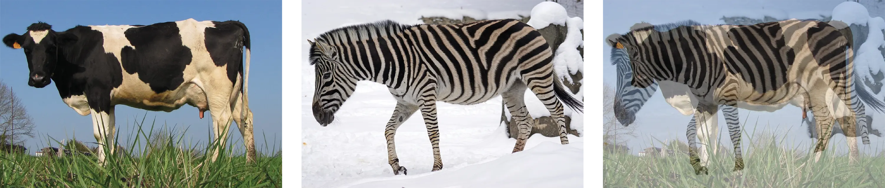
Blending is a way of combining numerical representations of multiple inputs to create new outputs that contain aspects of each input.

Two main approaches to blending data:

Content blending	Parametric blending
mixes raw data directly rather than underlying structure example: mixing images of a cow and a zebra result: a simple superposition of both images, not a meaningful "zebracow" hybrid	mixes the parameters that describe the underlying structure of objects example: blending the center, radius, and color of two circles result: an "in-between" circle with blended properties, something meaningful

However, parametric blending does not work well with arbitrary compressed representations, because compression can destroy the internal structure needed for meaningful interpolation.

Autoencoders solve this problem:

• they learn compressed representations that preserve important structure
• this allows parametric blending to produce meaningful blends

The simplest autoencoder

An autoencoder is a type of neural network that compresses data and then reconstructs it:

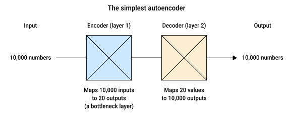
• input:
  • 100×100 pixels grayscale images of animals → 10,000 numbers
• encoder (layer 1):
  • maps 10,000 inputs → 20 outputs (called a bottleneck layer)
  • output is a compressed version of the image
  • these 20 outputs are called latent variables (they capture values inherent in the input data)
• decoder (layer 2):
  • maps 20 values → 10,000 outputs
  • tries to reconstruct the original image from the compressed data

This network is trained so that the output matches the input.

Since the input itself is the target, this is called semi-supervised learning (no labels, just the input data).

If trained on a single image (like a tiger):

• the autoencoder seems to compress and reconstruct it perfectly
• but this is overfitting: the network memorizes the image instead of learning general compression
• evidence: it outputs a tiger even for unrelated images, relying mostly on biases

Training on a larger set of images reveals the bottleneck's limitations:

• 20 latent values aren't enough to capture all the information
• as a result, reconstructions are blurry or inaccurate

A better autoencoder

To work well, an autoencoder needs:

1. enough latent dimensions to represent the data
2. enough computational capacity (neurons and layers) to encode and decode data effectively

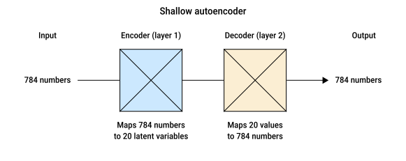
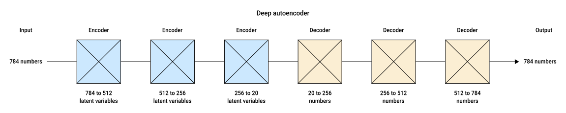
Below, we compare two autoencoder architectures using the MNIST dataset (60,000 labeled 28×28 grayscale images of handwritten digits).

Both models are trained for 50 epochs (= we run through all 60,000 samples 50 times).

Architecture	Explanation	Image
Shallow autoencoder	input: 28×28 image flattened into 784 values encoder: one fully connected "bottleneck" layer reducing 784 → 20 latent variables decoder: one fully connected layer expanding 20 → 784 (flattening layer at the start and unflattening layer at the end are omitted in the diagrams) result: reconstructed images are blurry but still recognizable
Deep autoencoder	input: 28×28 image flattened into 784 values encoder (3 fully connected layers): 784 → 512 latent variables 512 → 256 latent variables 256 → 20 latent variables decoder (3 fully connected layers): 20 → 256 numbers 256 → 512 numbers 512 → 784 numbers (these sizes commonly halve and then double, though this is a guideline, not a rule) result: produces much clearer reconstructions than the shallow 20-latent version

Exploring the autoencoder

A closer look at the latent variables

Latent variables are compressed representations of input data that encode the essential information needed to reconstruct inputs.

The network learns its own private encoding that makes little sense to humans.

For example, using the deep autoencoder seen above:

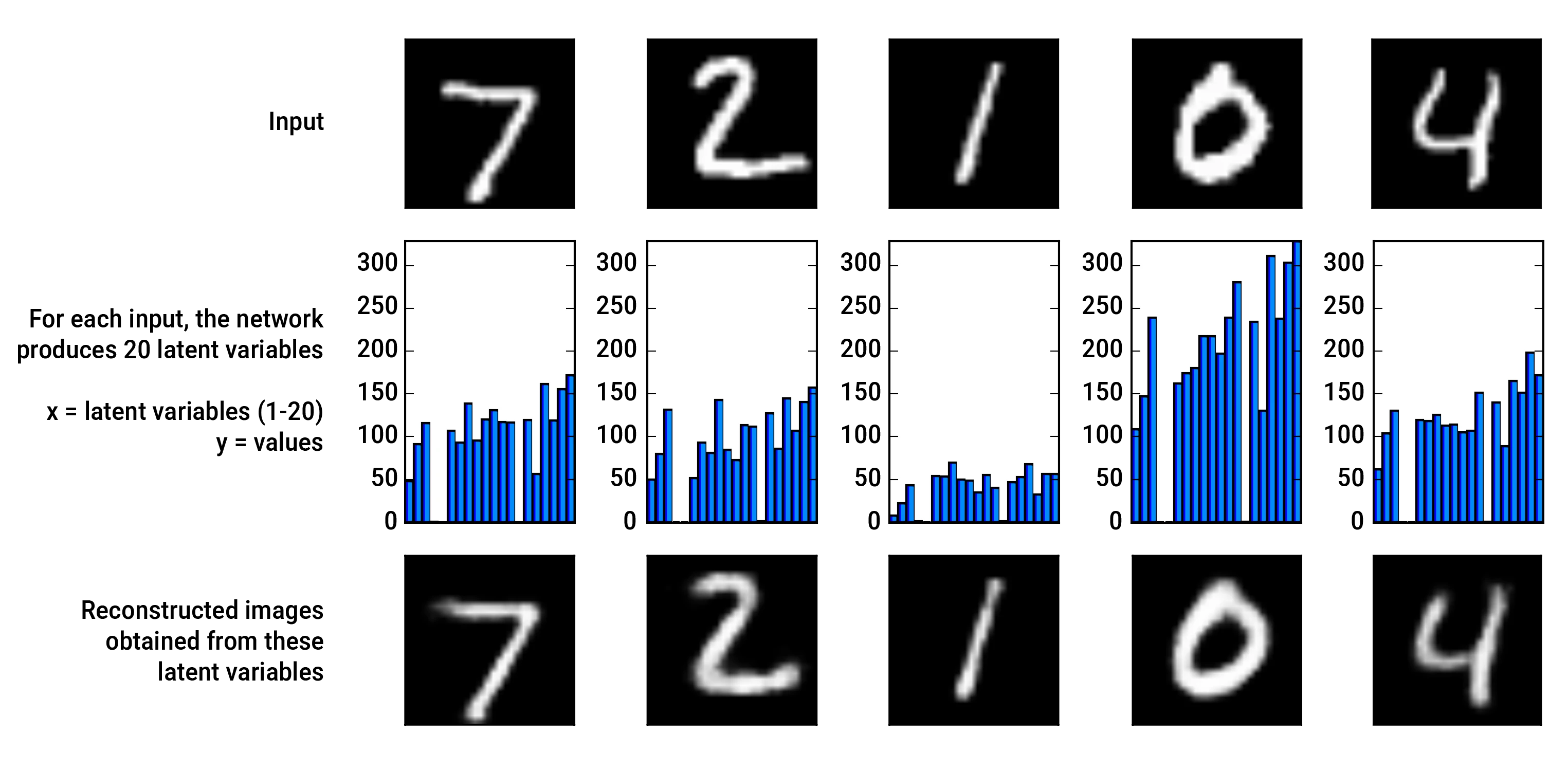
• for each input, the network compresses each one into just 20 latent variables shown as graphs:
  • x-axis = latent variables (1-20)
  • y-axis = value of latent variables
• different images produce different patterns
• some latent variables (like 4, 5, and 14) are consistently near zero across images, but there's no obvious reason for that
• e.g., you cannot say that latent variable 4 represents the top edge or latent variable 14 a curve on the left

This lack of interpretability is not a problem, because the latent variables serve as an internal code optimized for accurate reconstruction.

The parameter space

Latent variables are high-dimensional and abstract.

To understand what they represent, we can reduce the encoder to compress each input into just two numbers that capture its key features, allowing us to plot and visualize them as (x, y) points.

Plotting 10,000 MNIST images onto a 2D plane shows the latent variable space (or latent space):

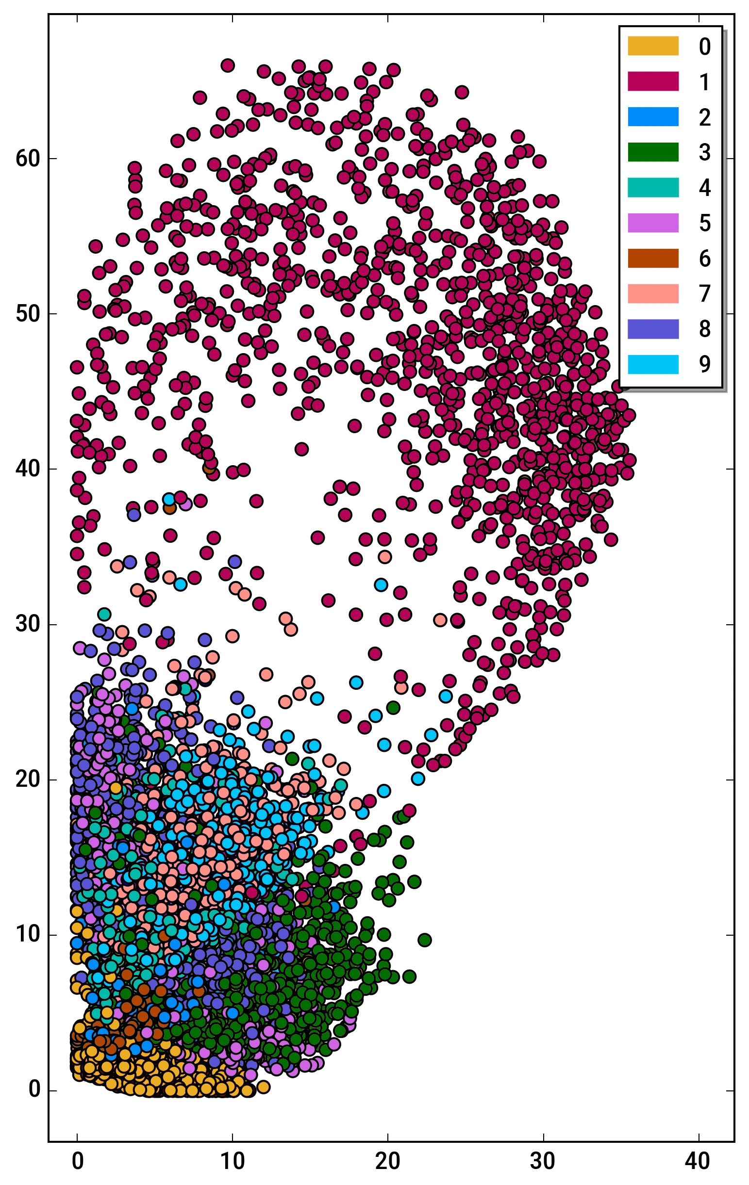
• x-axis = latent variable 1
• y-axis = latent variable 2
• each dot represents an image color-coded by the digit it represents
• similar images (like 1s, 3s, 0s) form clusters, as they are assigned similar latent values
• some overlap occurs in dense regions, meaning similar latent values can encode different digits

Decoding these 2D points back into images reveals what each region represents:

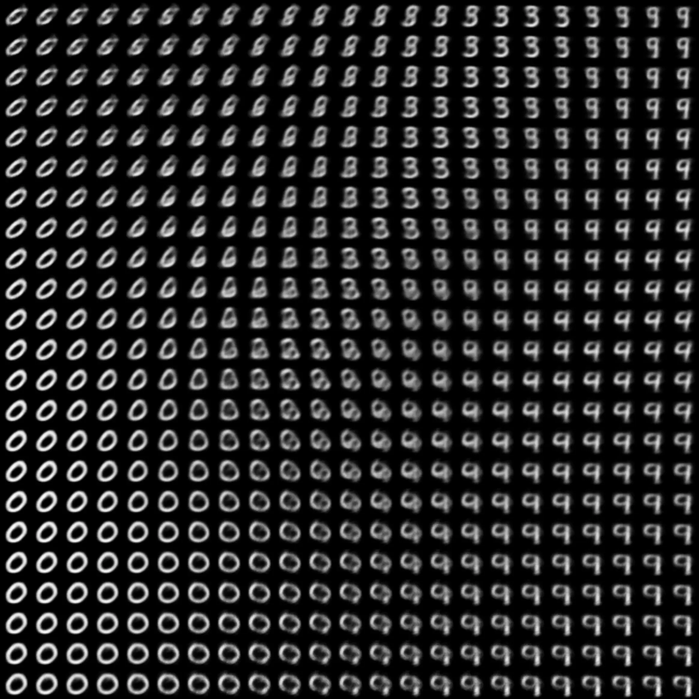
• using only two latent variables produces blurry images, but the structure is still meaningful
• autoencoders assign similar latent values to similar inputs, forming clusters
• adding more latent variables improves separation between clusters, but higher-dimensional spaces are impossible to visualize

Blending latent variables

Blending latent variables means mixing the compressed representations of two inputs so the decoder can create smooth intermediate outputs.

Intermediate outputs reveal relationships between points in the latent space.

Having more latent variables makes blended results more detailed and realistic.

Example using the 6-layer deep autoencoder:

• take the latent variables of:
  • image A [a1, a2, …, a20]
  • image B [b1, b2, …, b20]
• average each pair: (a1 + b1) / 2, (a2 + b2) / 2, … to create a new latent vector
• decode this new vector with the autoencoder to generate an intermediate image

Results:

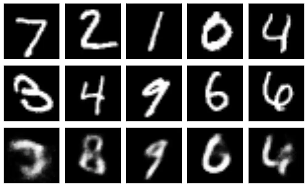
• intermediate images capture features of both originals, rather than simply overlaying them
• example: blending a "2" and "4" resemble a "8" because those digits are close in latent space

Limitations:

• some interpolated images do not resemble any digit or break into abstract shapes
• this occurs when blended latent points land in sparse or empty regions of latent space
• the decoder must guess what the image should look like, producing imperfect or unusual results

Predicting from novel input

Using the deep autoencoder trained on MNIST digits, we compress and decompress a tiger image, resized to 28×28 pixels to fit the network:

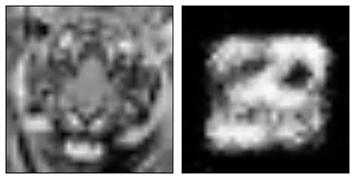
• since the autoencoder has never seen a tiger, it interprets the image as a digit
• the output is a mix of digit-like shapes and doesn't look like a tiger

This shows that autoencoders only work well on data similar to what they were trained on, because their latent variables are designed to represent that specific type of data.

Convolutional autoencoders

Since convolutional layers are well-suited for image data, they provide a natural way to build an autoencoder for MNIST.

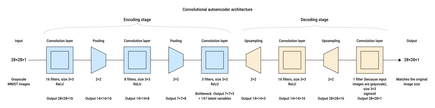
• encoder:
  • 3 convolutional layers
  • the first two are followed by 2×2 pooling
  • after the third convolution, the representation is reduced to a 7×7×3 tensor (the bottleneck)
• decoder:
  • uses upsampling and convolution
  • expands the bottleneck back to a 28×28×1 reconstructed image

Training this model for 50 epochs produces reconstructions that are very close to the original digits.

Blending the latent variables of two images, however, gives mixed results. The intermediate images are often messy because the network has never seen "between" digits during training.

The same limitation appears with out-of-distribution inputs. When given the low-resolution tiger image, the model cannot map it meaningfully into the digit-based latent space, so the output is not tiger-like.

Like simpler autoencoders, convolutional autoencoders cannot generalize to new inputs or latent-variable combinations that lie outside the data they were trained on.

Denoising

A popular use of autoencoders is to remove noise from images by learning to reconstruct clean data.

In this example, noise is added to images from the MNIST dataset:

• 
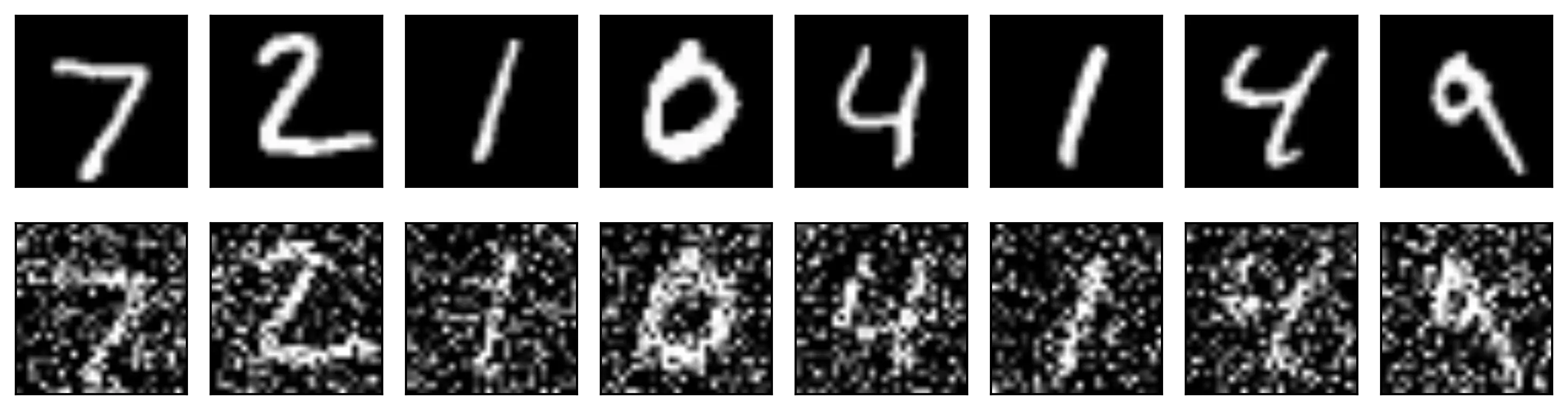
• random Gaussian noise (mean 0) is added to each pixel
• pixel values are forced to stay within the 0–1 range to keep the image within the valid grayscale range

The autoencoder is trained using noisy images as input and clean images as targets.

The model learns a latent representation that captures the underlying structure of the digits while ignoring random noise.

Two architectures are tested.

Model 1 - convolutional autoencoder with explicit downsampling and upsampling layers:

• the tensor (bottleneck) after the third encoding convolution contains 1,568 values (7×7×32)
  • this is larger than the input (28×28×1 = 784)
  • while inefficient for compression, this is acceptable because the goal is denoising rather than dimensionality reduction
• produces clean, high-quality reconstructions of the noisy digits

Model 2 - simplified architecture using only convolution layers:

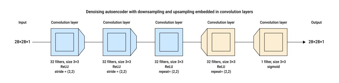
• follows modern design trends and uses only convolution layers:
  • strided convolutions for downsampling (first 2 layers)
  • repeated convolution for upsampling (last 2 layers)
• produces nearly identical denoising results while training about one-third faster
• 

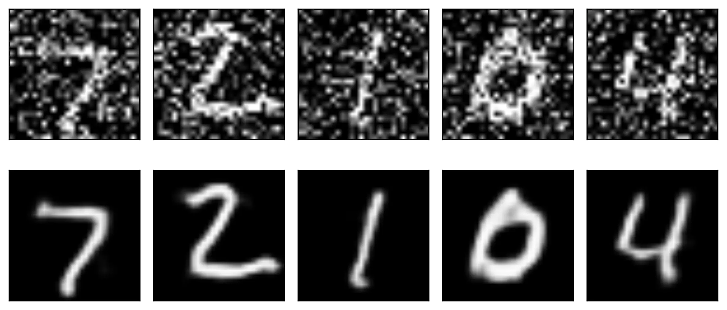
Both architectures work well for denoising, though determining which is better would require more detailed evaluation.

Variational autoencoders

Traditional autoencoders suffer from an unstructured latent space, where regions may be mixed or empty, leading to poor-quality outputs.

A Variational Autoencoder (VAE) addresses this by organizing the latent space more effectively:

• each class occupies its own distinct, non-overlapping zone
• large empty areas are minimized (though some are unavoidable due to limited data)

VAEs are nondeterministic, introducing randomness during encoding, so they don't always produce the same output for the same input.

Training

A Variational Autoencoder (VAE) is designed to generate realistic outputs from random latent variables by organizing the latent space during training.

To do this, it enforces three key properties:

1. all latent variables occupy a defined region (so we know where to sample when generating new data)
2. similar inputs produce latent variables that cluster together
3. empty regions in latent space are minimized

This structure is achieved using a specialized loss function that penalizes violations of these rules.

Clustering the latent variables

The specialized error term of VAEs encourages the values of each latent variable to follow a unit Gaussian distribution:

• latent variables cluster near the center (0), keeping them in a consistent region
• when generating new samples, choosing values from this Gaussian distribution:
  • keeps them close to what the model saw during training
  • leads to realistic, coherent outputs that resemble the training data

In practice, perfect Gaussians are rarely achieved:

• the VAE balances matching the Gaussian shape with accurately reconstructing data
• this balance is learned automatically during training

Clumping digits together

A VAE learns to group similar inputs in latent space.

For example:

• all handwritten 2s should cluster together
• finer variations (looped vs. unlooped, straight vs. curved, thick vs. thin, tall vs. short) should form their own sub-clusters

A high-dimensional latent space enables the model to group together all variations of these features.

The VAE discovers these features and groups the images automatically (no manual labeling needed).

In latent space, distance between latent vectors (points in multidimensional space) reflects how much two images resemble each other.

Training must balance two competing goals:

• keep similar images close together in latent space
• ensure latent variables follow a Gaussian distribution

To balance these goals, VAEs introduce randomness, letting the model "usually" cluster similar inputs while still keeping the Gaussian structure.

Introducing randomness

To generate varied outputs from similar inputs, a VAE introduces randomness into the latent variables produced by the encoder.

A simple idea:

• add small random numbers directly to the latent variables before sending them to the decoder
• this would:
  • produce different versions of the same input
  • help similar inputs cluster together in latent space
• but this randomness breaks backpropagation, because gradients cannot be computed through a purely random operation

VAEs solve this using the reparameterization trick:

• instead of adding random noise directly, the encoder outputs the parameters of a Gaussian distribution for each latent variable:
  1. a center (the mean μ) – where the latent value should be
  2. a spread (the standard deviation σ) – how much it can vary
• think of the encoder as saying: "For this input, the latent value should be roughly here, but it can wiggle this much"
• a random value is then sampled using: \( z = \mu + \sigma \cdot \epsilon, \quad \epsilon \sim N(0,1) \)
• this sampled value becomes the latent variable passed to the decoder
• this preserves randomness while allowing backpropagation:
  • randomness is kept, but it is now combined with the learned parameters (μ and σ) in a standard formula
  • because this formula is traceable, gradients can still flow through the network during training

Implementation requires splitting since the encoder must output two parameters (μ and σ) for each latent variable:

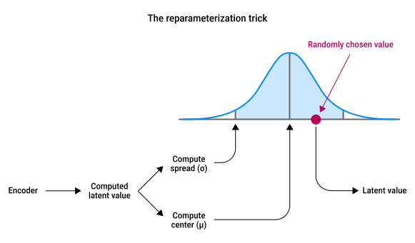
This is why trained VAEs are nondeterministic and give slightly different results every time: the encoder is deterministic up to the mean and standard deviation, but the sampling step introduces variation.

Exploring the VAE

A fully connected VAE is similar to a standard autoencoder with two key enhancements:

• the encoding stage ends with a split–select–merge step producing latent distributions
• the loss function combines (a) measuring reconstruction error with (b) KL divergence to decrease the differences between the encoder and decoder, ensuring the decoder can accurately reverse the encoder's transformations

Working with the MNIST samples

Using the above VAE to reconstruct MNIST digits demonstrates how the model encodes and generates data:

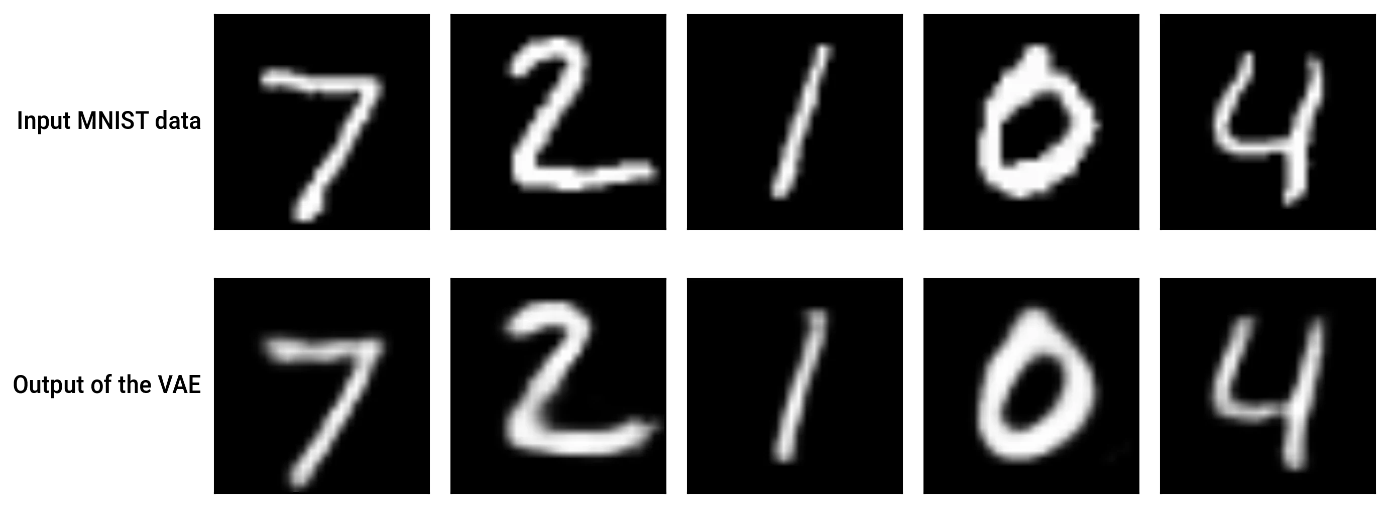
The VAE produces good matches of input digits, but because it samples from a latent distribution, the output varies for the same input:

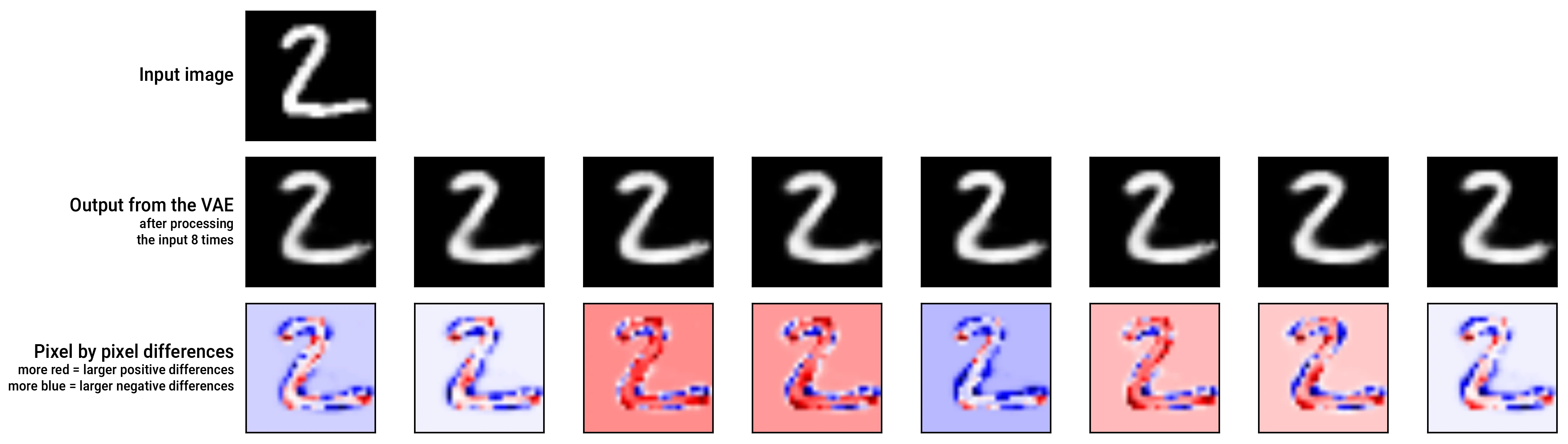
• the same input gives slightly different results each time
• pixel-difference images show where the reconstructions differ

The latent space is stable even when we add noise to test its structure:

• adding 10% noise to each latent variable (inside the bottleneck, after the encoder) hardly changes the output
• even 30% noise still produces recognizable digits
• this shows the latent space is well-structured, so nearby points map to valid digit shapes

Blending the latent variables of two images is used to test the continuity of latent space:

• produces coherent transitions between digits
• blended outputs look like reasonable digits or digit-like shapes
• this works because the latent space is smooth and densely populated, so intermediate points remain close to valid digit representations

Out-of-distribution inputs don't produce meaningful results:

• passing a non-MNIST image (a low-res tiger) through the VAE produces non-digit-like output
• VAEs only generate meaningful outputs for data similar to what they were trained on

Working with two latent variables

We trained a VAE with only 2 latent variables (instead of 20) to better visualize how it organizes the latent space.

Plotted latent variables for 10,000 MNIST images:

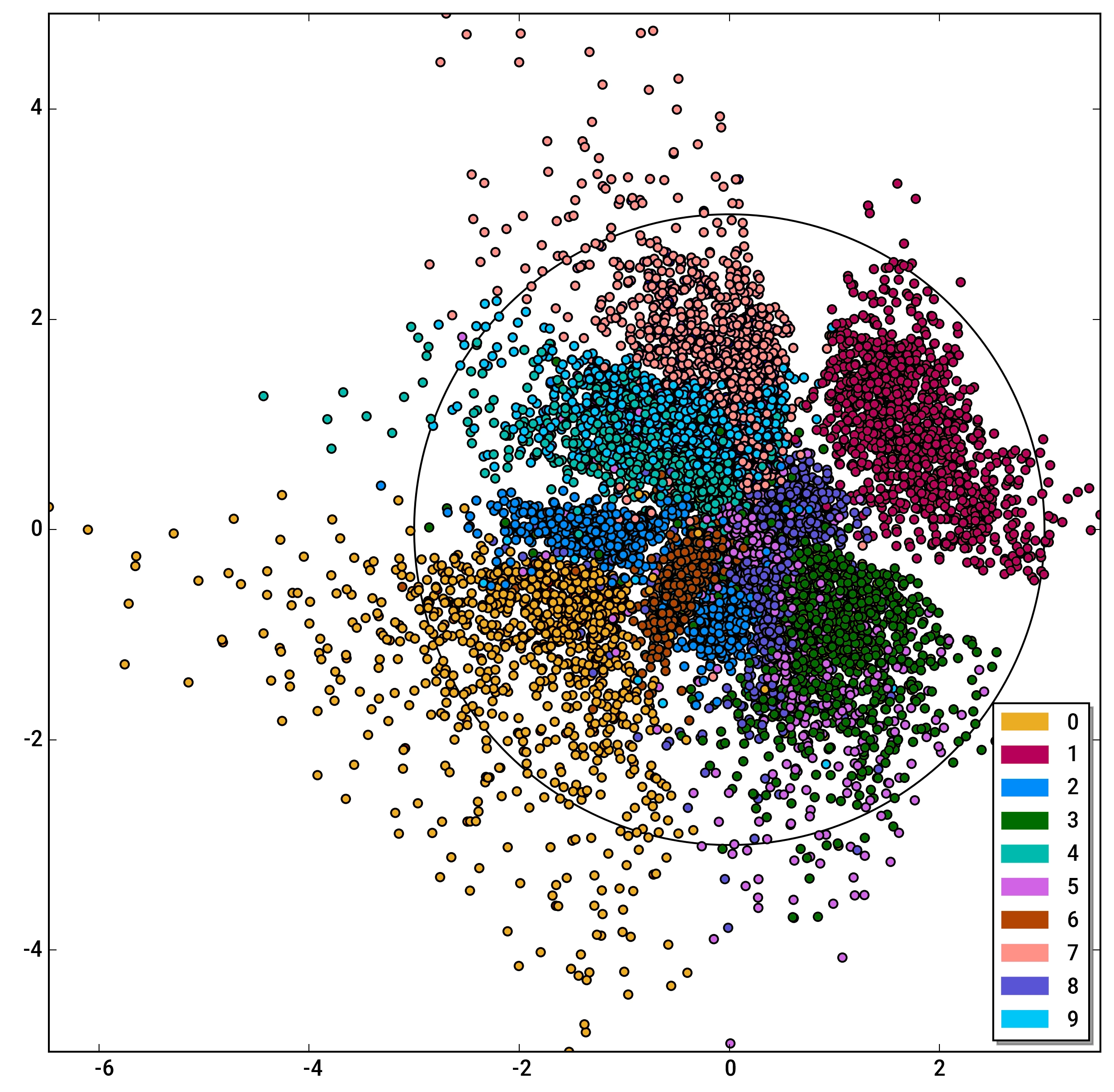
• the black circle shows the Gaussian bump the latent variables aim to stay within
• most digits cluster nicely, though there's some confusion near the center
• some digits, like "2", form two separate clusters

Decoding the latent space:

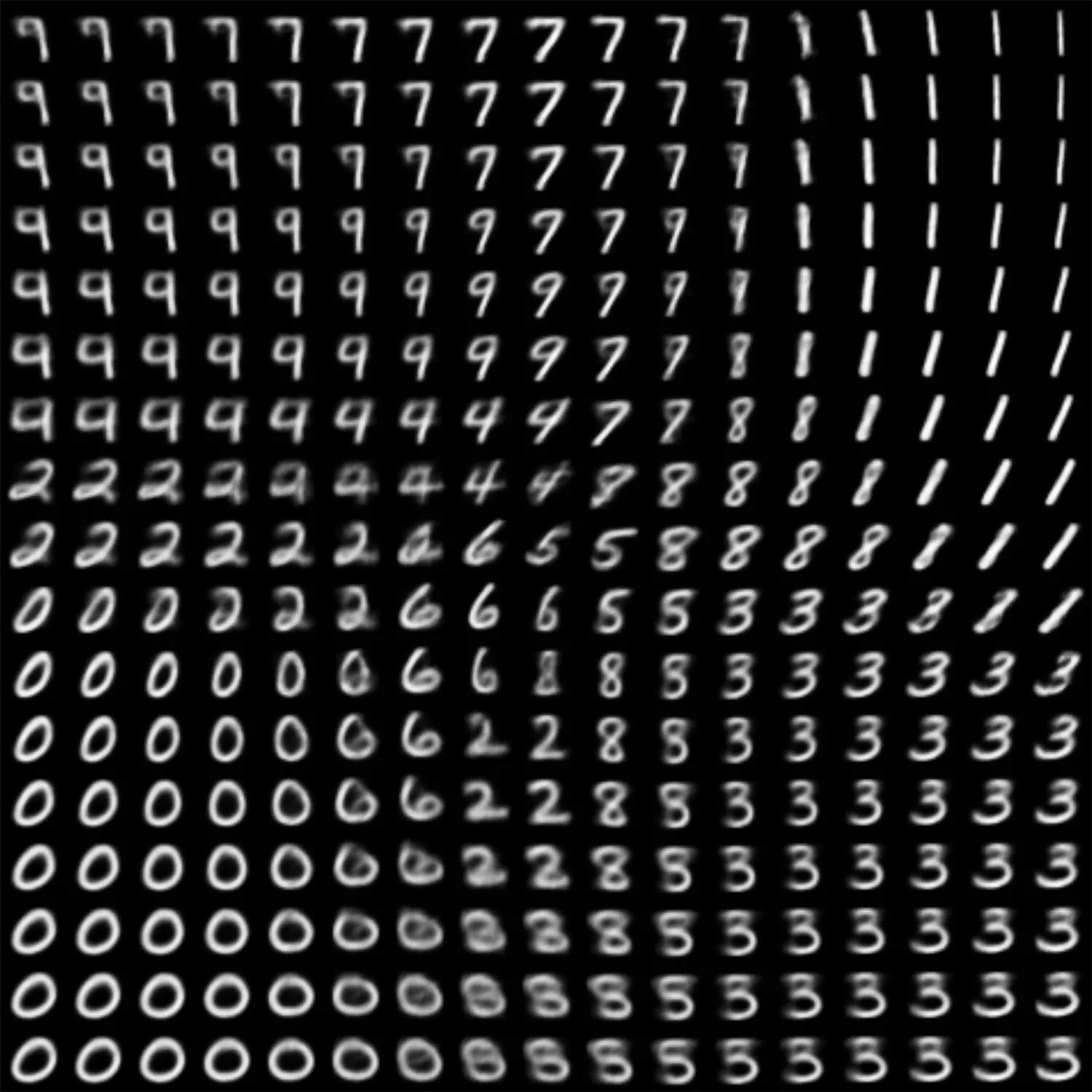
• we fed the x and y coordinates of each point to the decoder to generate images
• the model separates the "2s with loops" from "2s without loops"
• the system decided that they are so different that they don't need to be near each other

Even with just two latent variables, the digits are well-clumped and structured, much better than earlier visualizations. Some images are slightly fuzzy, but most still look digit-like.

Producing new input

A VAE can generate new images by:

• isolating the decoder after training
• feeding it random latent variables

The number of latent variables affects the output:

• with only two latent variables:
  • the generated digits are often fuzzy or ambiguous
• with 50 latent variables:
  • the generated digits are much sharper and more realistic
  • a few odd hybrid shapes still appear, likely from mixed or empty regions in the latent space

Once trained, the decoder can be used on its own as a generator to create unlimited new images.

This approach works for any type of data the VAE has been trained on.