Convnets in practice

Categorizing handwritten digits

The MNIST dataset contains 60,000 grayscale images of handwritten digits (0–9), each sized 28×28 pixels.

The task is to identify the digit shown in each image.

A simple convnet designed for this job (implemented in the Keras library):

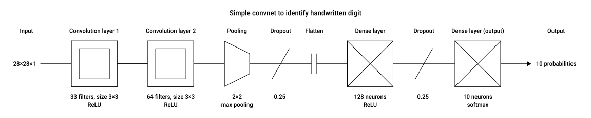
1. input: 28×28×1 grayscale image
2. convolution layer 1:
   • runs 32 filters (3×3x1)
   • each filter's output passes through a ReLU activation function
   • stride = 1
   • no padding → loses a ring of values around the edges (but fine because MNIST digits have a 4-pixel black border)
   • output tensor: 26×26×32 (32 filters = 32 channels)
3. convolution layer 2:
   • runs 64 filters (3×3x32)
   • ReLU activation
   • no padding
   • output tensor: 24×24×64
4. max pooling (2×2)
   • downsamples the feature maps by taking the maximum value in each 2×2 block
   • output tensor: 12×12×64
5. dropout (diagonal slash)
   • randomly disables 25% of neurons in the previous layer
6. flatten (two parallel lines)
   • we're switching from convolutional layers to fully connected layers which require a list as input
   • flatten takes all the values in the tensor and puts them in order into a long list
   • 
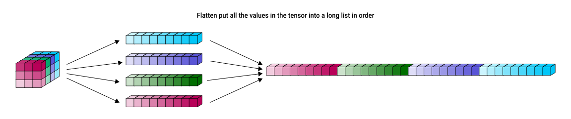
   • output vector: 12×12×64 = 9,216 values
7. dense (or fully connected) layer:
   • 128 neurons
   • ReLU activation
   • produces 128 outputs
8. dropout (diagonal slash)
   • randomly disables 25% of neurons in the previous layer
9. dense layer (output):
   • 10 neurons (one per digit) produce 10 outputs
   • softmax converts outputs to probabilities to get the final digit prediction

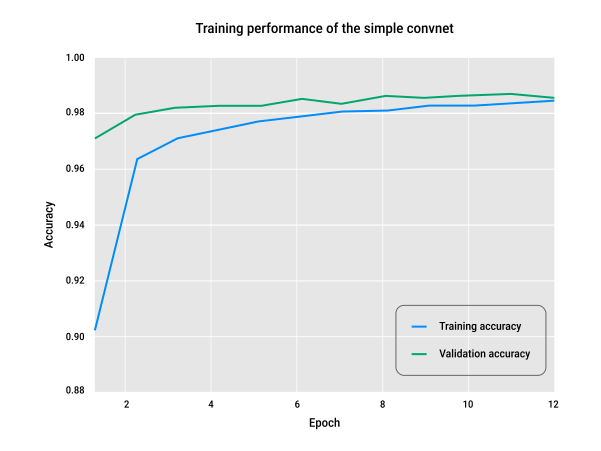
• trained for 12 epochs
• achieves ~99% accuracy on both training and validation sets
• no overfitting (training and validation curves are close)
• achieves this high accuracy with only two convolution layers

VGG16

VGG16:

• convolutional neural network developed by the Visual Geometry Group
• trained to analyze color photographs and identify the dominant object by assigning probabilities to 1,000 classes
• won an image-classification task at ILSVRC 2014, trained on 1.2 million labeled images across 1,000 categories (ImageNet dataset)

To use the model, input images must be preprocessed exactly like the original training data:

• resize images to 224×224×3 (RGB)
• each RGB channel has a specific mean value subtracted from all its pixels (see original VGG16 paper)

Architecture:

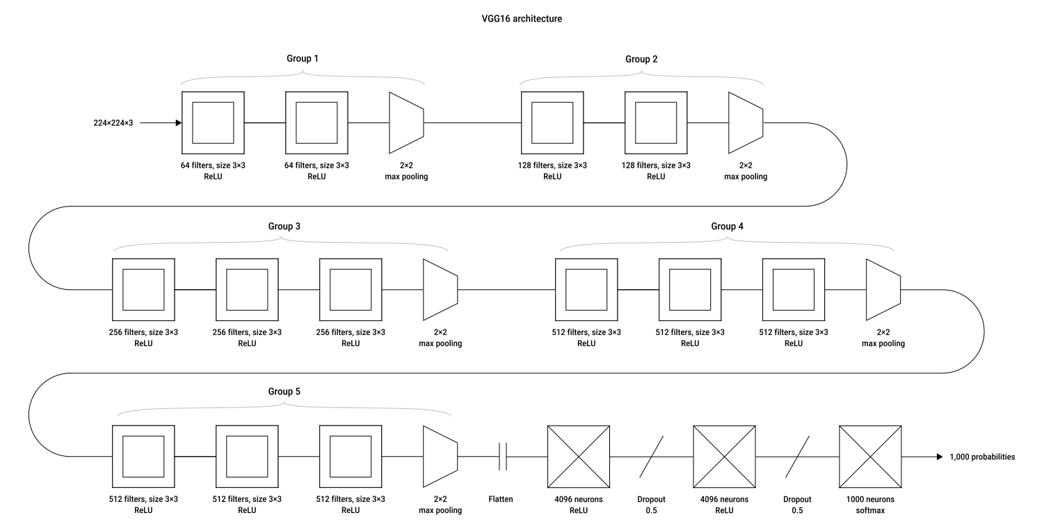
• 16 main layers (mostly convolutional)
• layers grouped for clarity, with each group ending in a pooling layer
• fully connected layers at the end

Layer-by-layer explanation:

1. input:
   • 224×224×3 RGB image
2. convolution layers:
   • group 1
     • apply 64 3×3 filters (with zero padding → no loss in width or height) + ReLU
     • apply 64 3×3 filters again (with zero padding) + ReLU
     • apply 2×2 max pooling
     • output tensor: 112×112×64
   • group 2
     • double the number of filters from Group 1
     • apply 128 3×3 filters
     • apply 128 3×3 filters again
     • apply 2×2 max pooling
     • output tensor: 56×56×128
   • group 3
     • double the number of filters again
     • apply 256 3×3 filters
     • apply 256 3×3 filters again
     • apply 256 3×3 filters a third time
     • apply 2×2 max pooling
     • output tensor: 28×28×256
   • group 4
     • apply three 3×3 convolution layers, each with 512 filters
     • apply 2×2 max pooling
     • output tensor: 28×28×512
   • group 5
     • apply three more 3×3 convolution layers, each with 512 filters
     • apply 2×2 max pooling
     • output tensor: 14×14×512
3. fully connected layers:
   • flatten
     • convert the 14×14×512 tensor into a 1-D list
   • dense layers
     • dense layer with 4,096 units → ReLU → 50% dropout
     • another dense layer with 4,096 units → ReLU → 50% dropout
     • dense layer with 1,000 neurons
   • softmax
     • produces a probability distribution over 1,000 categories

Performance:

• VGG16 performs extremely well, even on new images it has never seen
• VGG16 remains popular as a starting point for image classification projects because it performs well, has a simple architecture, and offers publicly available pretrained weights

Visualizing filters, part 1

VGG16's success is due to the filters learned by its convolutional layers.

Since each filter is just a large array of numbers, it's hard to interpret them directly.

Instead, we can visualize what a filter has learned by creating an image that activates it as strongly as possible.

To do this, the usual training process is reversed:

1. pick a filter you want to understand
2. use gradient ascent:
   • normally, gradient descent updates the weights to reduce error
   • here, we reverse the idea:
     • freeze all the network's weights
     • change only the input image
     • adjust the pixel values in the direction that increases the filter's output
3. feed a random image into the network
4. measure the chosen filter's output (the feature map):
   • if the filter sees information that it's looking for, it produces large activation values
   • add up all the values in that feature map
   • use this sum to compute the gradients
5. backpropagate gradients to the input image (not to the weights)
6. adjust input pixels repeatedly to increase the filter's activation:
   • with each iteration, the random image becomes better at activating the filter
7. result:
   • the final image strongly excites the chosen filter, revealing the kind of pattern it has learned to detect
   • because the process starts from random pixels, running it multiple times produces slightly different images, but they all share similar patterns since they maximize the same filter

Images that maximally activate the filters (saturation enhanced for easier interpretation):

Chosen filters	Comment	Image
Group 1 → Layer 2 → All 64 filters	Early filters detect simple edges and orientations.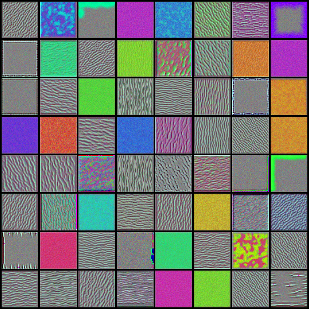
Group 3 → Layer 1 → First 64 filters	Middle filters detect more complex textures formed from earlier features.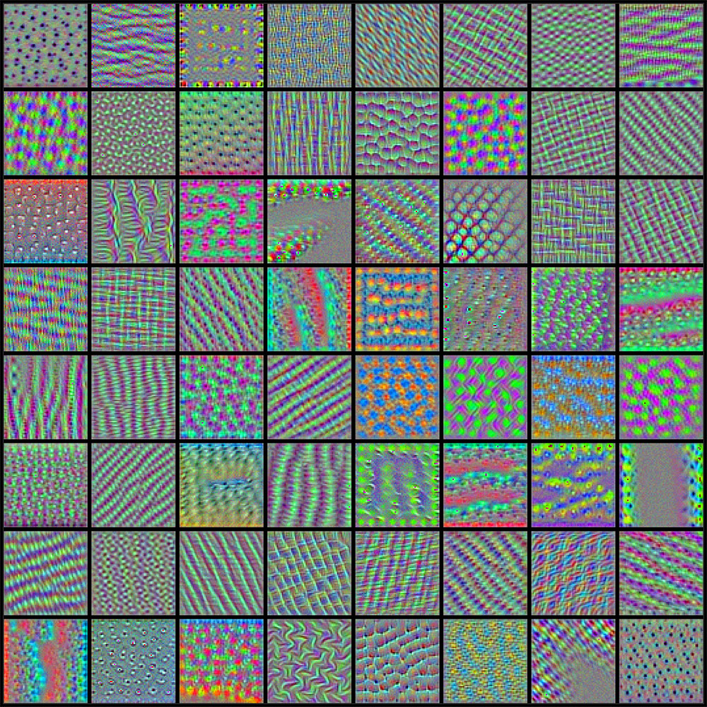
Group 4 → Layer 1 → First 64 filters	Deeper filters capture intricate, organic textures resembling those found in natural images (likely influenced by ImageNet containing many images of animals).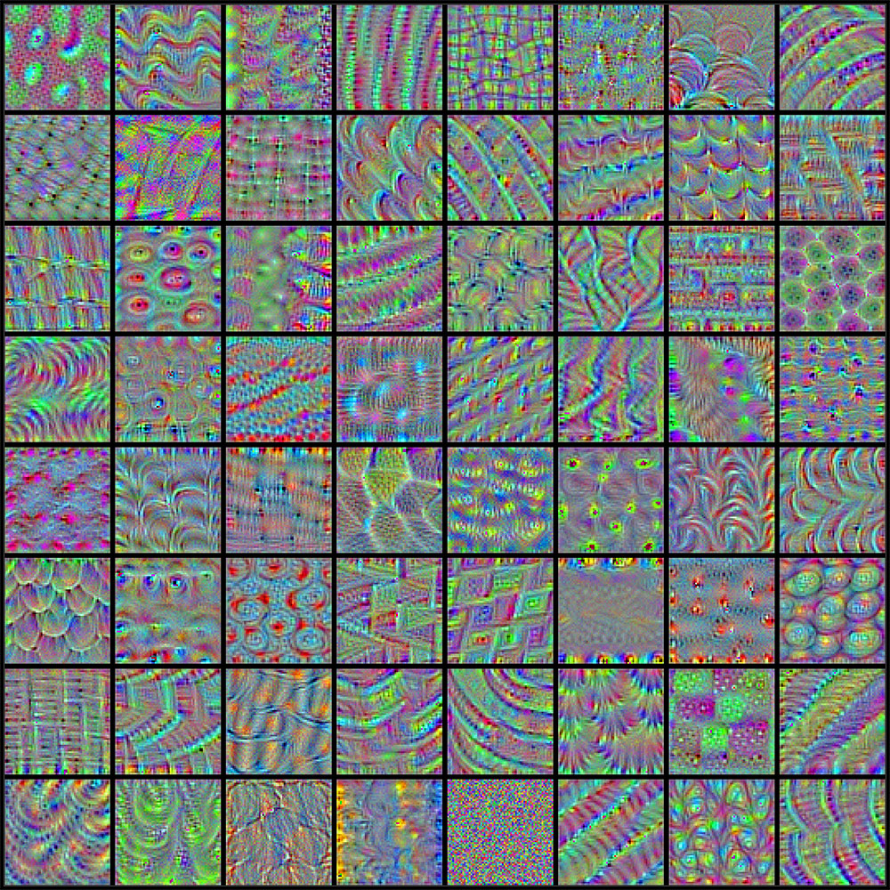

The convolutional hierarchy allows filters to progress from detecting simple edges to capturing rich, high-level textures.

Visualizing filters, part 2

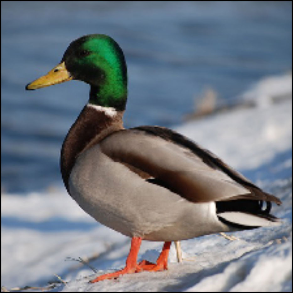
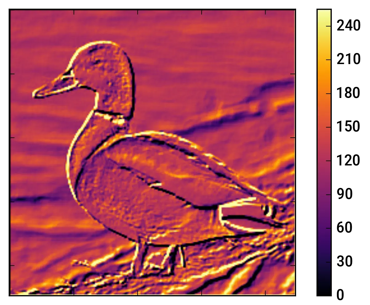
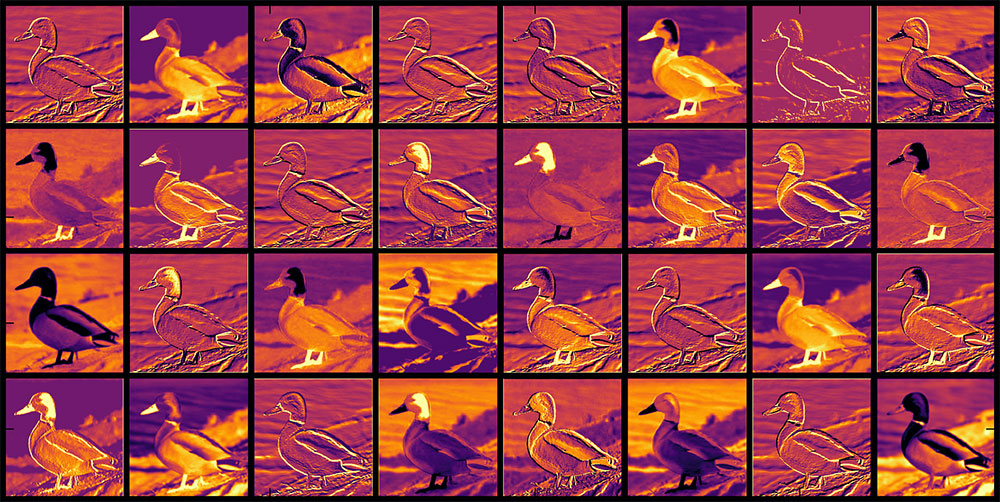
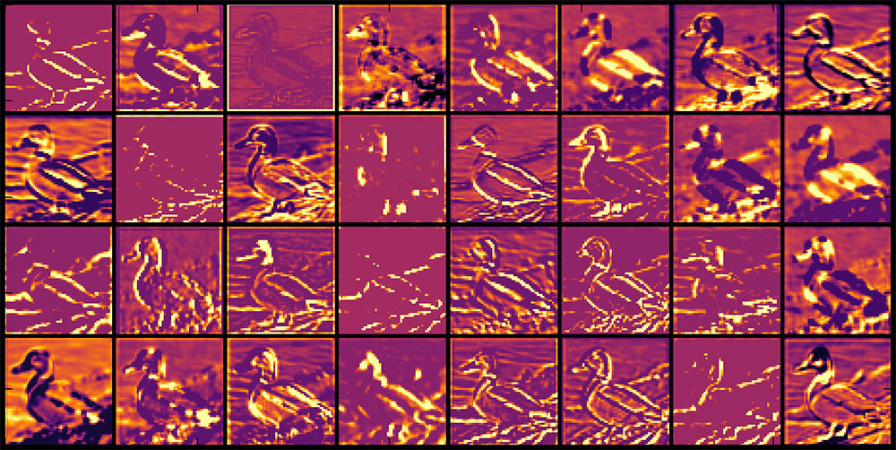
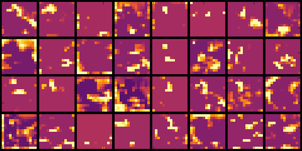
Another way to visualize a CNN filter is to look at its feature map (what it outputs for a particular image):

1. feed an image into VGG16
2. extract the feature map produced by the filter you want to examine
3. since each feature map has a single channel, it can be displayed as a grayscale image

Below are examples using:

• an RGB duck image as input
• feature maps shown as a heatmap instead of grayscale for easier interpretation

Chosen filter(s)	Comment	Image
Group 1 → Layer 1 → Filter 0	the filter acts like an edge detector edges that are light trigger strong activation areas of constant color give medium responses
Group 1 → Layer 1 → First 32 filters response	many filters detect edges others respond to simple visual patterns, like colors or textures
Group 3 → Layer 1 → First 32 filters response	feature maps are 4× smaller in each dimension (due to pooling layers) many filters still act as edge detectors, meaning edges remain important cues for VGG16 some filters activate strongly for more complex patterns
Group 5 → Layer 1 → First 32 filters response	feature maps are even smaller (due to pooling layers) the duck is barely recognizable (features have become highly abstract) many filters combine earlier features into high-level concepts some filters barely activate because they detect features not present in the duck image

Adversaries

Even though VGG16 can accurately classify images, almost invisible changes can completely mislead the network.

For example:

• adding a very small modification to an image can cause VGG16 to misclassify it
• these modified images are called adversaries, created by adding an adversarial perturbation

Some perturbations are universal: a single perturbation can fool a classifier on many or even all images, not just one.

Example: a tiger image is altered by a very small perturbation:

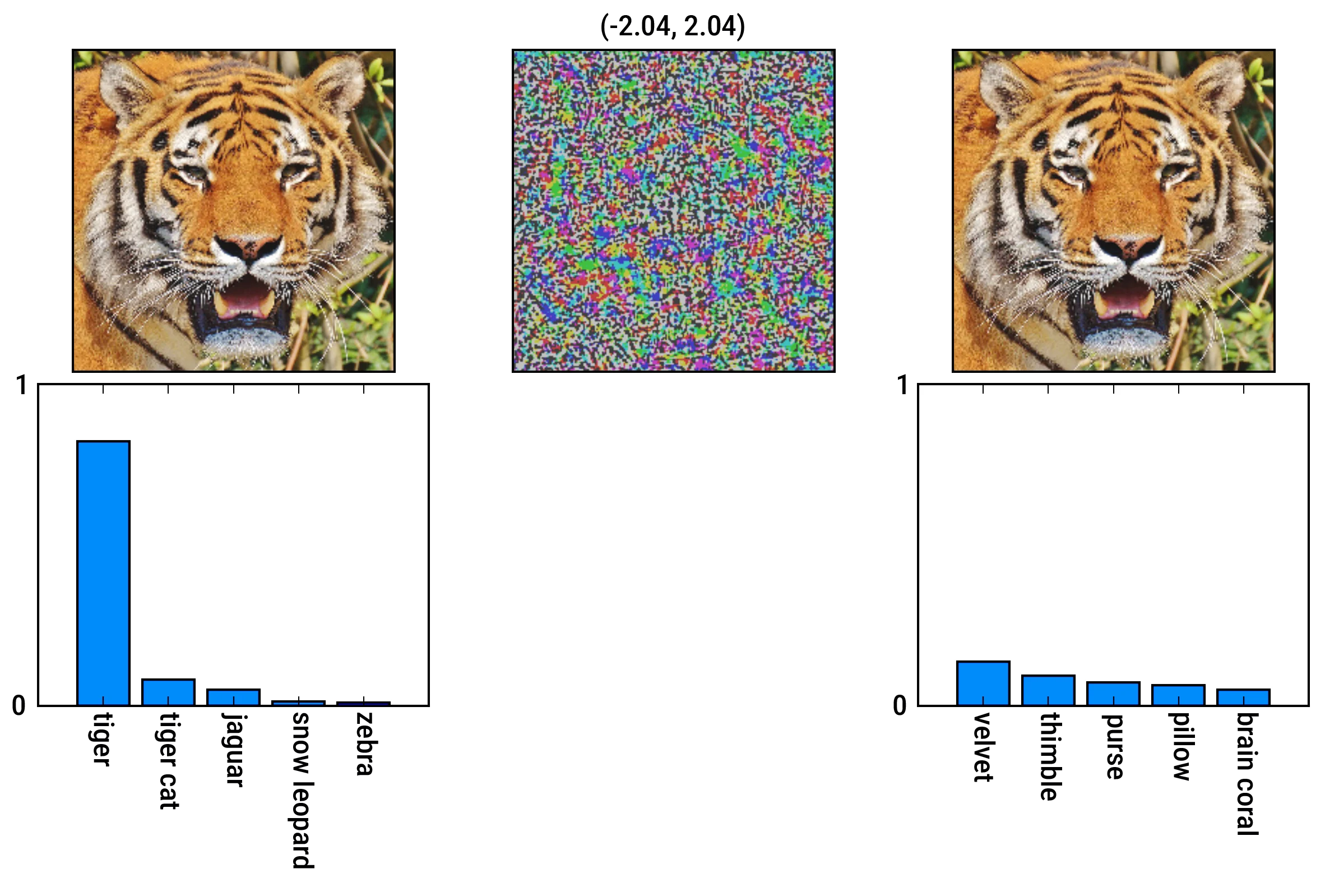
• original: correctly classified as a tiger
• perturbation: values in [-2, 2] (shown here scaled to [0, 255] for visibility)
• result: the image looks unchanged to humans, but the classifier's predictions become completely wrong

There are many ways to generate adversarial perturbation:

• various algorithms produce perturbations of different sizes
• some aim for any misclassification
• others force a specific wrong label
• some attacks suppress the network's top predictions rather than aiming for a specific class

These attacks exploit subtle vulnerabilities in convnets and show that we still don't fully understand their internal behavior.