Convolutional neural networks

Convolutional neural networks (CNNs) or convnets are a deep learning technique based on convolution.

CNNs learn to "see" the world of their inputs.

Introducing convolution

Detecting yellow

A convolutional filter (or kernel) is a set of weights used in a CNN to detect a specific feature from an input.

Example - detecting yellow in a color image:

Step	Explanation	Image
Input	RGB image. Each pixel has 3 values: R, G, B ∈ [0,1].
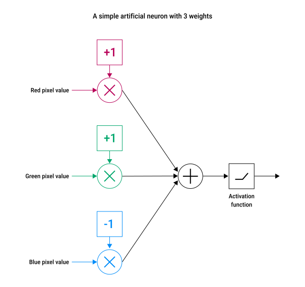
Yellow detector (neuron)	Compute a yellowness score per pixel: yellow ≈ high R, high G, low B (1, 1, 0) detection can be done using a neuron with 3 weights: (+1, +1, −1) for (R, G, B) these 3 weights form a kernel (+1, +1, −1) Kernel size = 1×1×3: size = 1×1 (because it looks at 1 pixel at a time) depth = 3 (because each pixel has 3 channels)
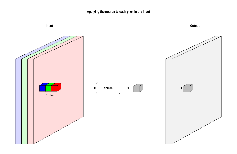
Apply to the whole image	The neuron is applied by moving pixel by pixel, row by row across the image. At each pixel: output = (+1 × Red) + (+1 × Green) + (−1 × Blue) This produces a new image (or tensor): same width and height but only one channel
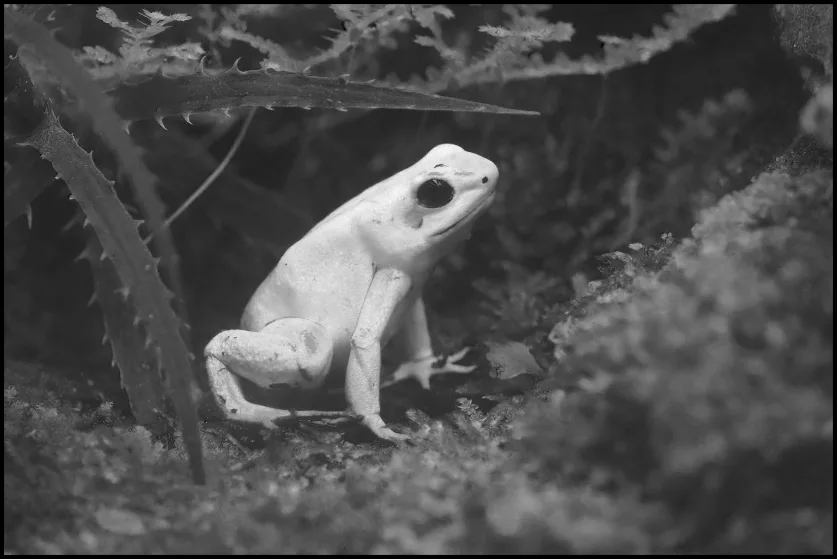
Output	If a pixel is very yellow, the output is large. In a grayscale image: larger numbers → brighter pixels → closer to white. So whiter pixels = more yellow in the input.

The sliding (or scanning, or sweeping) operation is called convolution (the mathematical operation).

In CNNs, convolution refers to sliding a learned kernel across an input and computing weighted sums at each position to produce feature maps. This enables detection of specific features (such as yellow).

Weight sharing

Weight sharing means all neurons use the same filter (set of weights) stored in shared memory:

• saves memory
• enables parallel processing by allowing GPUs to compute many pixels simultaneously
• allows easy adjustments (changing the shared weights updates all neurons)

Especially useful in CNNs, since convolutions apply the same filter across many positions in an input.

Larger filters

The area of pixels a filter "sees" is called its local receptive field or footprint:

• 1×1 filter neuron → footprint = 1 pixel
• 3×3 filter neuron → footprint = 3×3 pixels

A filter with a footprint larger than one pixel is called a spatial filter.

When convolving across the image, the center of the filter is called the anchor or reference point.

Filters can be any size, but small odd-numbered squares (1×1 to 9×9) are most common to keep the anchor centered.

Filters and features

Neuroscience suggests that our visual system doesn't just send all visual data to the brain to process.

Instead, some early pattern recognition happens right in the eyes:

• certain neurons act as "feature detectors" — they fire only when they see specific shapes or movements
• for example, some neurons respond to particular lines or edges

In CNNs, filters (or feature detectors) mimic this process by scanning images for features (or patterns) like edges, lines, or textures.

The output of a filter is a feature map, showing how well each part of the image matches the filter.

Example - detecting vertical stripes:

Step	Explanation	Image
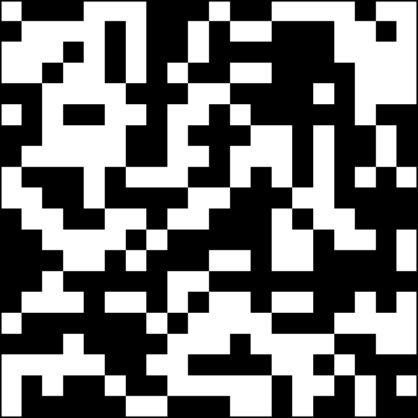
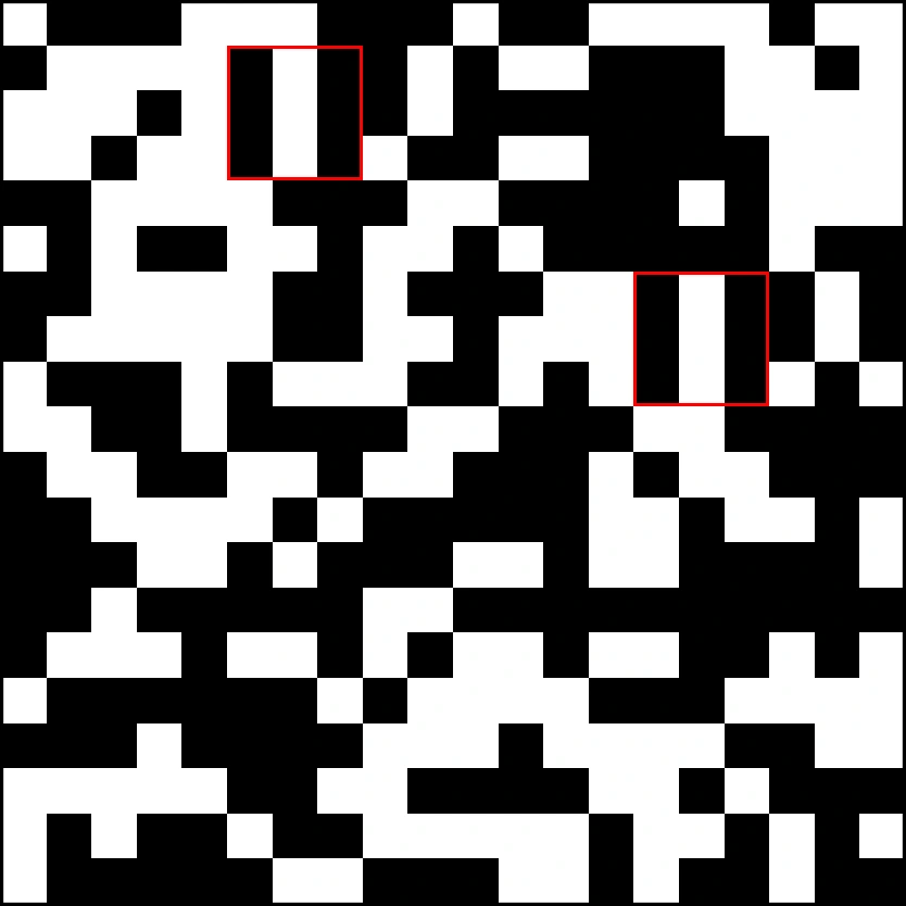
Input	Binary 20×20 image with values 0 (black) and 1 (white).
Filter (Kernel)	3×3 filter designed to detect vertical white stripes, with values -1 (black) and 1 (white).
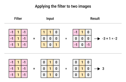
Apply the kernel	Slide the filter one pixel at a time over the image. At each position, multiply the filter values by the pixels beneath it and sum the results to produce one single output value.
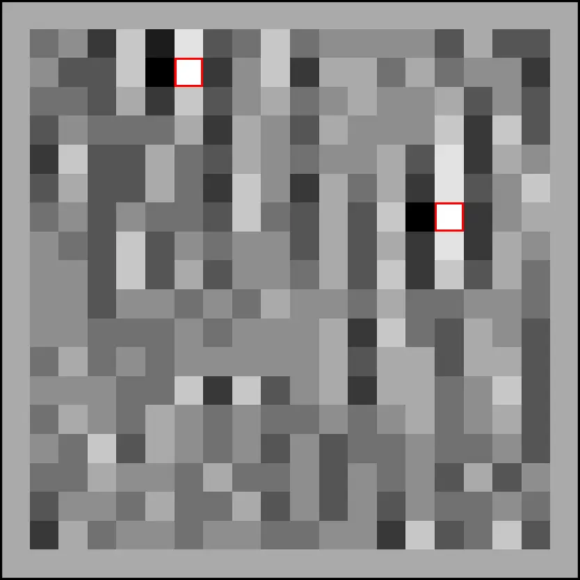
Result = feature map	Sliding a 3×3 filter across a 20×20 image one pixel at a time produces 18 positions where the filter fully fits (in both width and height), so the resulting feature map has size = 18×18. The feature map shows match strength with values from -6 to 3 (scaled to [0,1] for display). Higher (whiter) values = better matches. Pixels with perfect matches +3 are highlighted with a red border.
	Areas of the input where those matches occurred highlighted with a red border.

CNNs learn filter weights automatically during training:

• they start with random filter weights
• adjust them via backpropagation and gradient descent to reduce error
• over time, the filters learn to detect the patterns that help classify images correctly

The fact that this process works and achieves high accuracy across many tasks is one of the great discoveries in deep learning.

Padding

When a convolution filter reaches the edge of an image, part of its receptive field can fall off the side. There are no pixels there, but we still need an output value.

Simply avoiding edges reduces the output size and loses information.

Padding solves this:

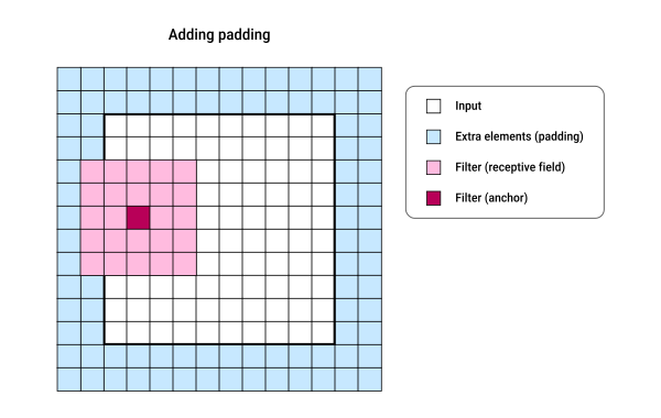
• it adds a border around the input so the filter can cover every pixel
• the border is filled with a constant value (usually 0) → "zero-padding"
• this lets the filter be centered on edge pixels without losing data
• this keeps the output width and height the same as the input

Multidimensional convolution

A convolution filter must have the same number of channels as the input tensor it is applied to.

This ensures that every input value is paired with a filter value:

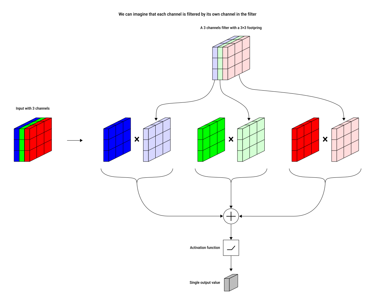
• the input image has 3 channels per pixel (red, green, and blue)
• the filter has 3 channels and a 3×3 spatial footprint, giving 27 total values
• during convolution, the filter is placed over a region of the image, and each value in the input block is multiplied with its corresponding value in the filter, across all channels

The process generalizes to tensors with any number of channels.

Convolution layers

A convolution layer consists of multiple filters (often hundreds) applied independently to an input tensor.

Each filter scans the same input independently to detect different features (like vertical lines, horizontal lines, or dots).

Each filter produces a single-channel feature map, and these outputs are stacked together to form the final output tensor.

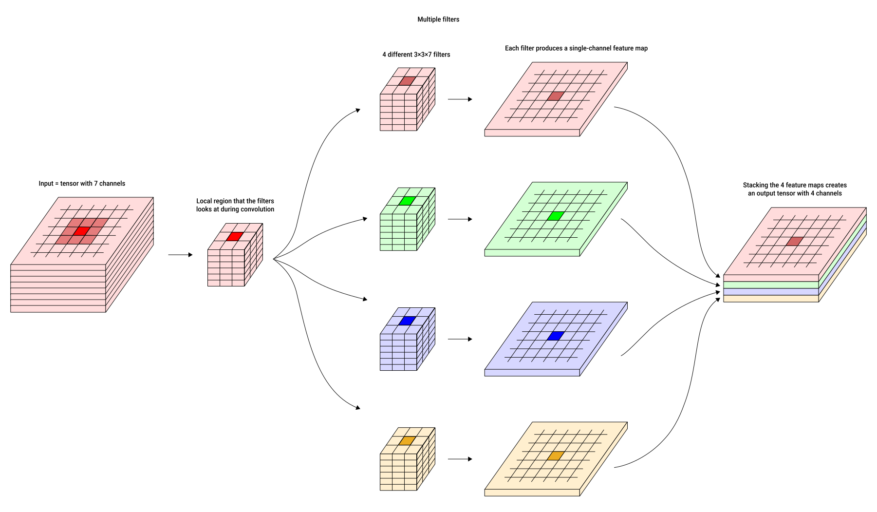
• input: tensor with 7 channels
• filters:
  • 4 different filters, each with a 3×3 spatial footprint
  • because the input has 7 channels, each filter must also have 7 channels
  • so each filter is a 3×3×7 tensor
• process: each filter produces a single-channel feature map
• result: stacking the 4 feature maps creates an output tensor with 4 channels

Main rules:

• each filter's number of channels must match the input's number of channels
• the number of output channels equals the number of filters used

Special types of convolution layer

1D convolution

In a 1D convolution layer, multiple filters move in only one direction (height or width).

It's often used in text processing, where data can be represented as a grid of letters or words.

Each filter covers the entire width (or height) of the input and slides along the other dimension.

1x1 convolutions (reducing the number of channels)

1×1 convolutions are used to reduce the number of channels in a tensor while preserving its spatial dimensions (width and height).

It works with multiple 1×1 filters:

• each 1×1 filter processes each spatial location independently and learns how to combine information across channels
• the number of channels in the output equals the number of filters used

The network automatically learns the best way to combine the input channels during training.

Reducing channels from 300 → 175:

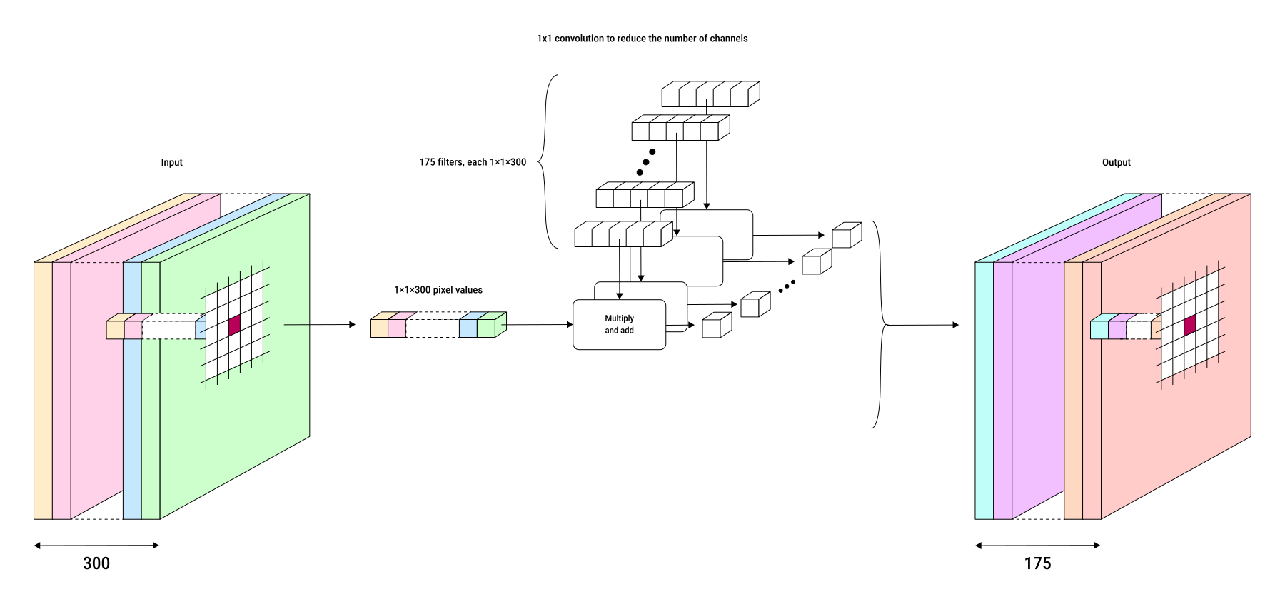
• input: a tensor with 300 channels
• 1x1 convolutions: use fewer 1x1 filters than the number of input channels
• output: a tensor with 175 channels, width and height remain the same

Benefits:

• useful when multiple channels contain redundant or overlapping information
• enables on-the-fly data compression inside the network (instead of pre-processing)
• reduces computation and memory usage by combining correlated or redundant features

Changing output size

In addition to the number of channels, width and height of a tensor can also be reduced to save computing resources.

Pooling (downsampling)

Reducing tensor size is a useful side effect of pooling, though its main role is robust feature detection if the input is slightly shifted.

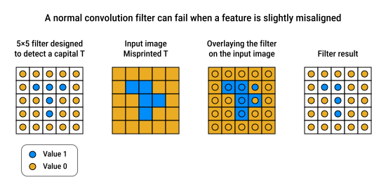
• one part of the filter does not find a matching blue pixel in the input
• so the filter reports no match
• if the filter could "look around", it could notice the nearby displaced blue pixel and match the input

The mathematical way to make the filter "see more" is to make the input image a bit blurry:

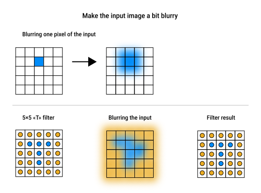
• the input is blurred, not the filters themselves, because this would interfere with training
• this allows slightly shifted features to be detected

Pooling is a method for blurring (or downsampling) a tensor by reducing its size.

Two types of pooling:

1. average pooling:
   • replaces each block with its average value
2. max pooling:
   • replaces each block with its largest value
   • networks using max pooling tend to learn faster since this preserves the strongest feature in each block
   • "pooling" usually means max pooling

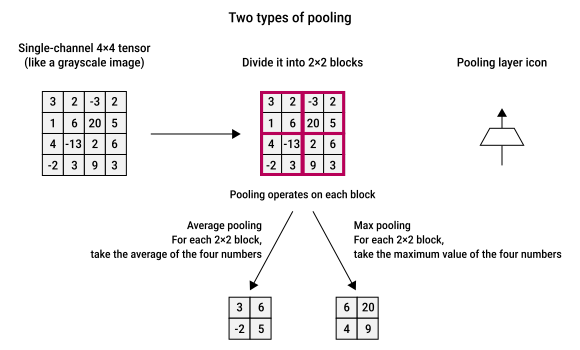
Pooling becomes useful when applying multiple convolution layers in succession:

• if the first filter's values aren't in the expected locations
• pooling helps by blurring or summarizing each region, so the next layer can still detect the pattern

When a tensor has multiple channels, pooling is applied separately to each channel:

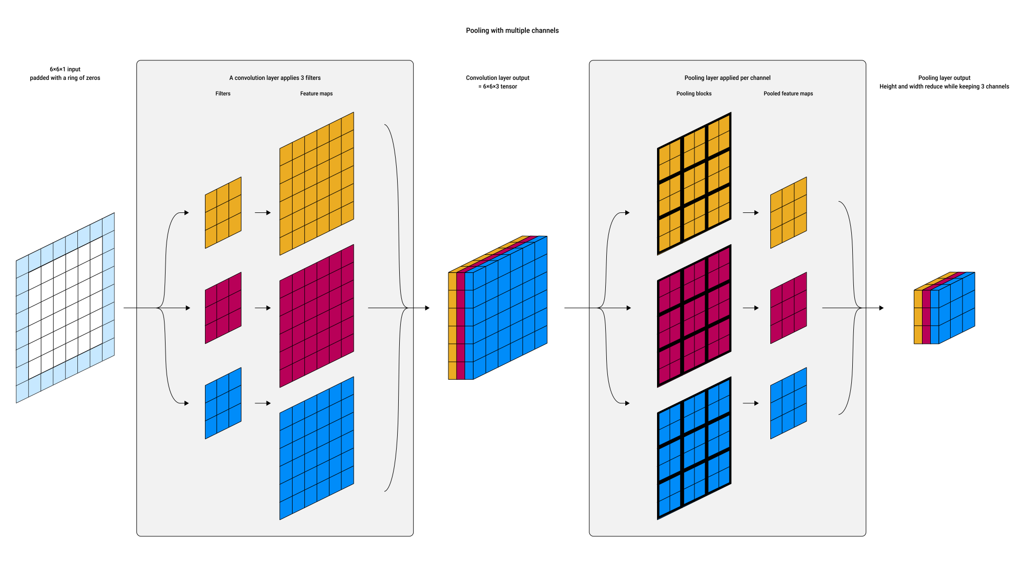
Pooling makes convolutions shift-invariant because it allows features to be detected even when their positions shift slightly.

Striding (downsampling)

Striding is the process of moving a convolutional filter by more than one pixel at a time (e.g., stride = 2), both horizontally and vertically, which reduces the output size.

Strided convolution is faster than convolution followed by a separate pooling layer because:

1. fewer filter evaluations
   • the filter is applied fewer times compared to moving one pixel at a time and then pooling
   • this reduces the total number of computations
2. no separate pooling step
   • strided convolution reduces output size directly, combining convolution and downsampling in one step

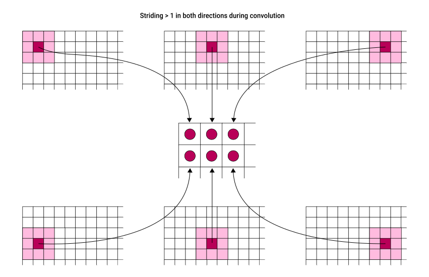
• instead of moving one pixel at a time, the filter skips multiple pixels
• it moves 3 pixels to the right on each horizontal step
• it moves 2 pixels down on each vertical step
• this skipping reduces the total number of positions where the filter is applied, which produces a smaller output tensor than the input

Depending on the stride, some input pixels may be reused, or each pixel may be used only once.

Strided convolution can replace pooling for downsampling, often producing similar results faster, because it avoids extra pooling computations.

However, the learned filters differ, so they can't be swapped one for the other without retraining.

Transposed convolution (upsampling)

Spatial dimensions can also be increased while keeping the same number of channels.

Standard upsampling simply repeats the input values as many times as we request.

Transposed convolution instead works by inserting zeros between and around input elements, then applying a convolution filter:

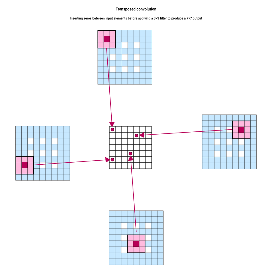
• input: a 3×3 image (shown as white squares)
• insert zeros between pixels (shown in blue)
• insert zeros around the outside (optional)
• apply a 3×3 convolution filter (shown in red)
• the result has dimensions 7×7

There is a limit to how much we can increase the input size. In practice, models double resolution using a 3×3 transposed convolution.

The output of transposed convolution is not identical to the result of upsampling followed by convolution because the operations behave differently mathematically.

Transposed convolution upsamples feature maps while preserving learned patterns, making it useful for e.g., image generation, segmentation, and decoding in autoencoders.

Hierarchies of filters

Convolutional networks, like biological visual systems, work in hierarchies of processing layers.

Each layer looks for patterns that are a bit more complex than the layer before.

To demonstrate this, we'll build a CNN to recognize simple binary faces with some simplifications:

1. images and filters are binary (only 0s and 1s)
2. filters look for exact matches
3. filters are hand-designed instead of learned
4. no padding is used (to keep diagrams simple)
5. use very small images (12×12) (so diagrams fit on the page)

Finding face masks

The recognition task is to determine whether a new image (the candidate) matches a reference mask even if small parts are slightly shifted.

A direct pixel-by-pixel comparison fails when the candidate differs slightly, even though the overall structure of the face is clearly the same:

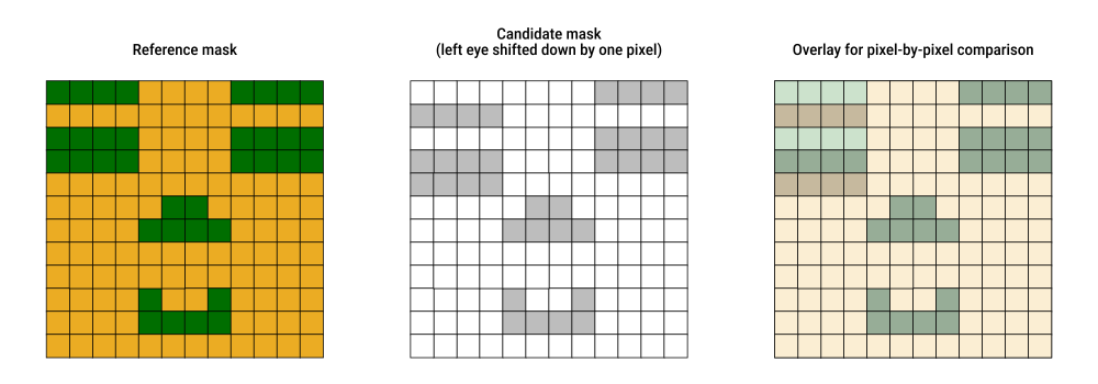
Instead, we can use convolution filters to check for structural similarity by detecting features and their arrangements.

Because it's easier to work backward, we start by designing the final filter:

• the goal is to identify a whole face containing:
  • one eye in each upper corner
  • a nose in the center
  • a mouth below the nose
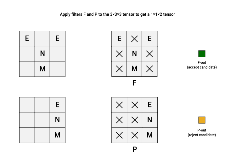
• this arrangement fits in a 3×3 grid
• challenge: binary filters use only 1 and 0 and cannot represent multiple feature types in one layer
• solution: use a 3-channel filter:
  • channel 1 = eye locations
  • channel 2 = nose locations
  • channel 3 = mouth locations
• combined, this gives a 3×3×3 tensor

This face detection filter (labeled F) can support different arrangements. For example, we create another filter (labeled P) that detects a face in profile:

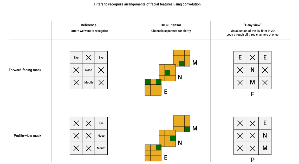
• cells marked with x mean that anything can appear there
• "X-ray view" = look through all channels and shows which channels have 1 in that cell

Finding eyes, noses, and mouths

Because the final filter detects eyes, a nose, and a mouth (3×3×3), the previous layer must produce those features arranged in a 3×3 grid.

For 12×12 input images, one approach is to use large 4×4 filters (E4, N4, M4) to detect eyes, noses, and mouths:

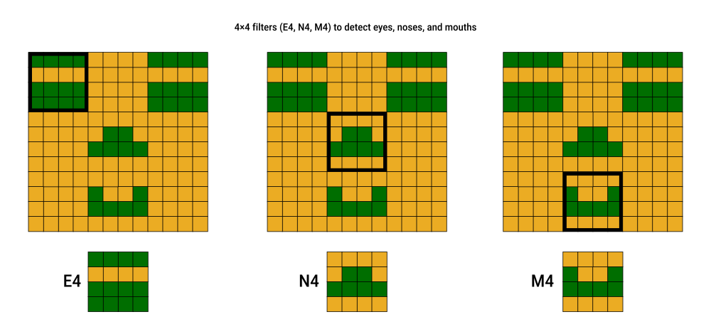
• without padding and assuming stride = 1, outputs are 10×10
• pooling reduces them to 3×3 for the final filter

However, this is computationally expensive and inflexible for detecting new features.

A more efficient and flexible approach is to use an additional convolution layer to build the 4×4 filters from smaller 2×2 blocks:

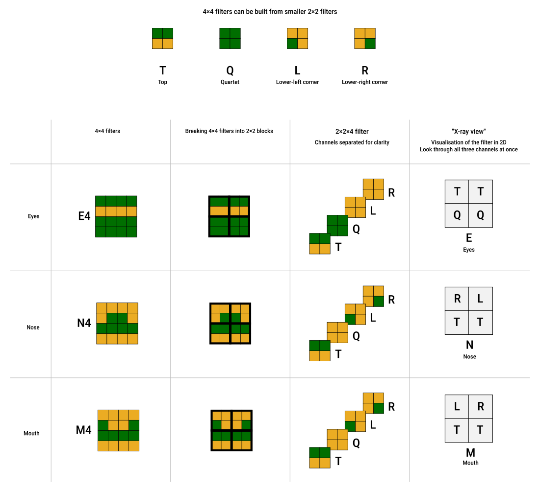
• top: four basic 2×2 filters acting as building blocks
• bottom: constructing the 4×4 filters of the additional convolution layer

Stacking filters

Stacking these filters produces a series of convolution layers where each layer uses the output of the layer below it:

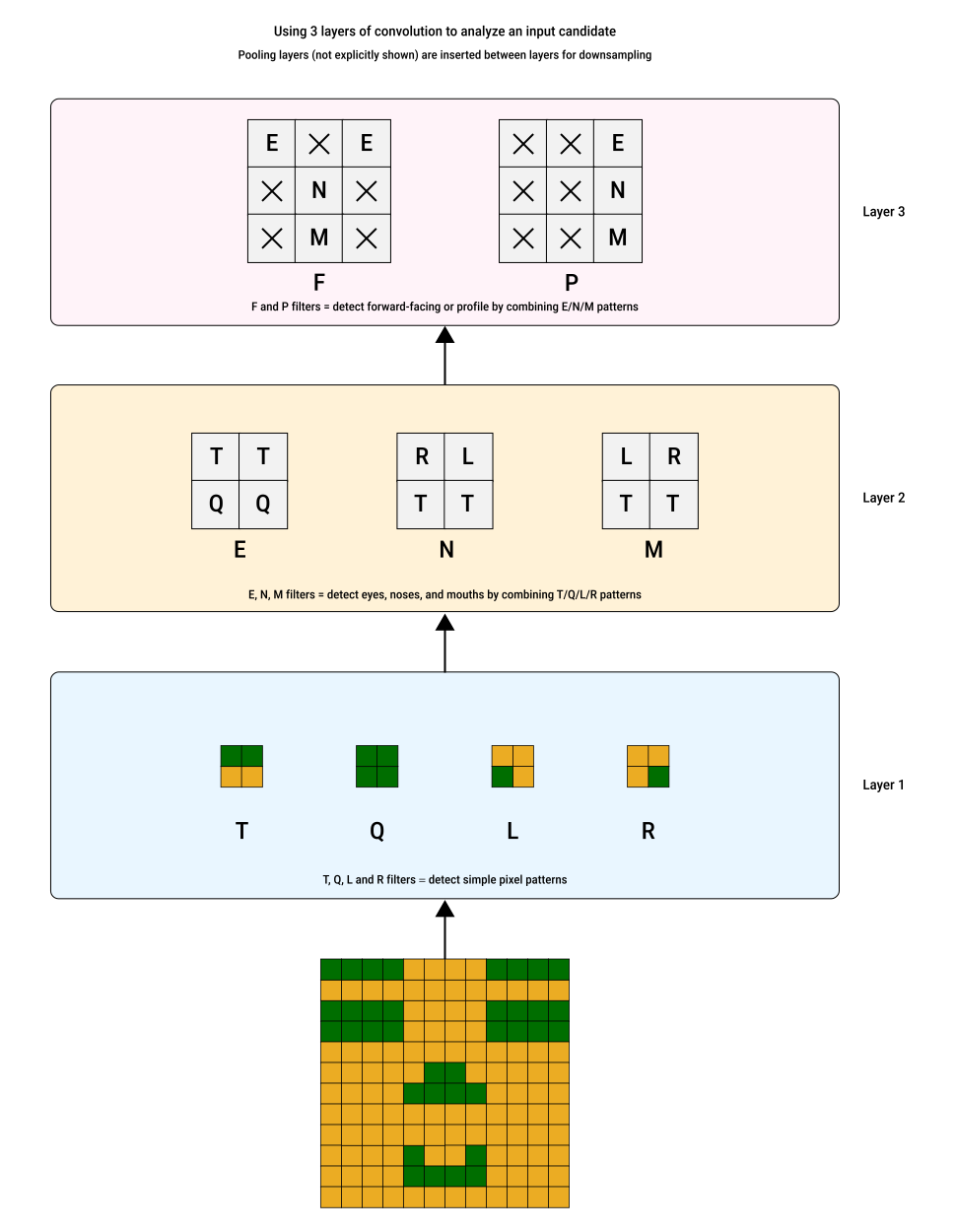
This hierarchical design is efficient (smaller filters reduce computation) and flexible (new features can be added without rebuilding large filters).

Applying filters

The overall result is an all-convolutional network (because all layers use convolution plus pooling):

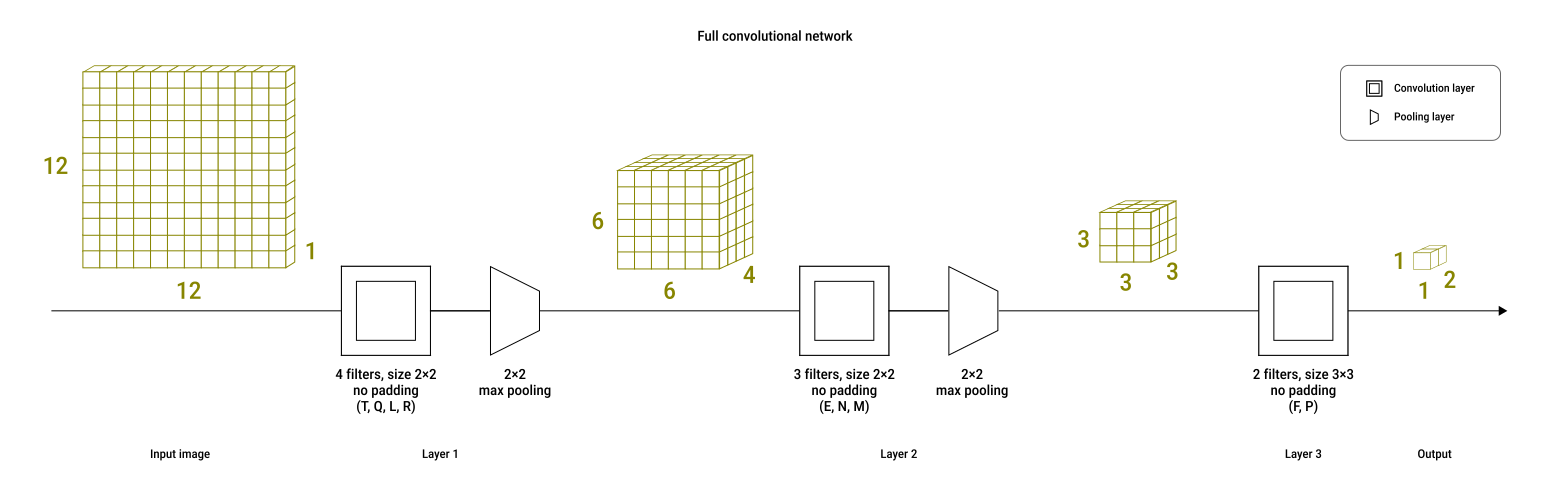
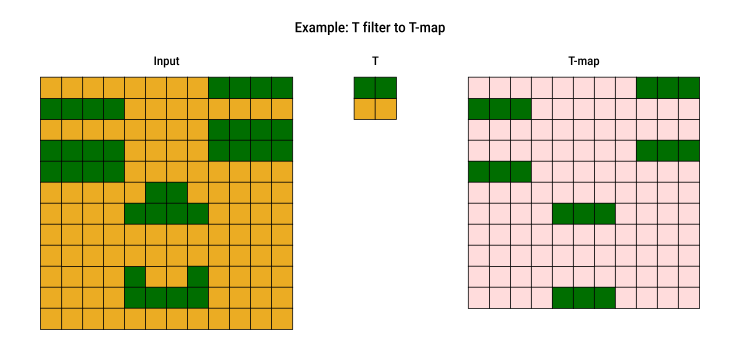
A candidate image is evaluated using three hierarchical layers.

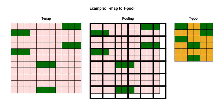
Pooling plays a key role by allowing robustness to small positional changes and reducing computation and memory use.

Step	Explanation	Image
Layer 1 — detecting basic patterns	Apply 2×2 filters T, Q, L, R to the 12×12 input image → T-map, Q-map, L-map, R-map no padding → convolving 1 pixel at a time produces 11×11 feature maps matches = 1 (green), non-matches = 0 (pink)
	Apply 2×2 max pooling to each feature map → T-pool, Q-pool, L-pool, R-pool each 2×2 block becomes 1 if there is any green inside output size becomes 6×6
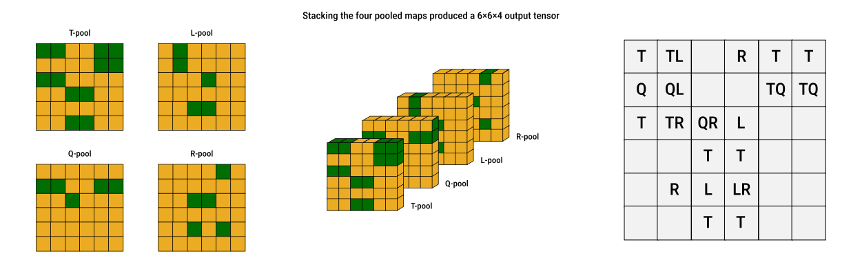
	Stack the four pooled maps → 6×6×4 output tensor
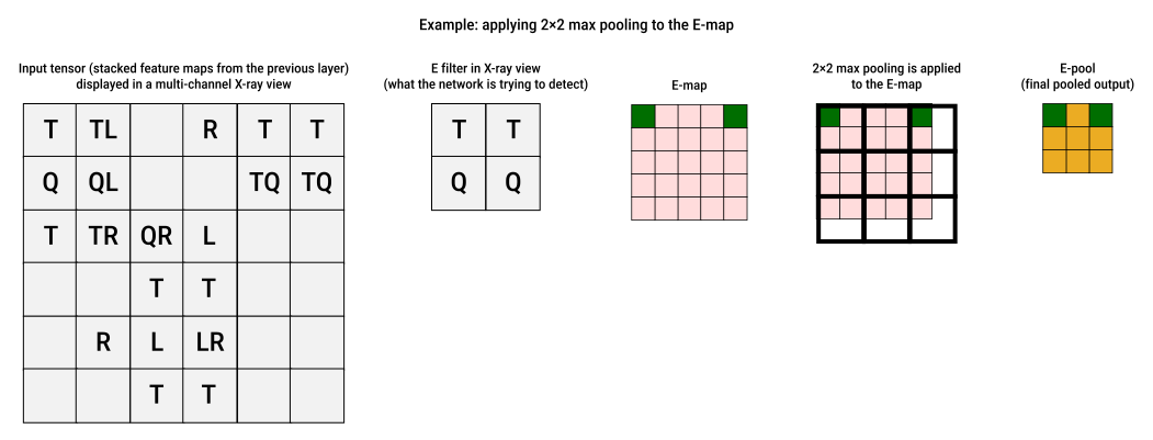
Layer 2 — detecting higher-level patterns	Apply filters E, N, M to the 6×6×4 tensor → E-map, N-map, M-map
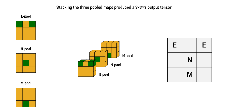
	Apply 2×2 max pooling to each feature map → E-pool, N-pool, M-pool. Pooling shrinks them to 3×3.
	Stack the 3 pooled maps → 3×3×3 output tensor.
Layer 3 — detecting whole-face patterns	Apply filters F and P to the 3×3×3 tensor: filters are the same size as the input (3×3×3), so they don't slide direct application produces a 1×1×2 tensor
Interpret the 1×1×2 tensor output	1st channel → result of the F filter (F-out) green → F matches → accept candidate beige → reject candidate 2nd channel → result of the P filter (P-out) green → P matches → accept candidate beige → reject candidate

By stacking convolution layers hierarchically, networks detect increasingly complex patterns:

• outputs of simple filters are fed into new filters to build complexity step by step
• first layers find basic features (edges, corners, colors)
• next layers combine those into more complex shapes (eyes, wheels, feathers)
• deeper layers recognize whole objects (faces, cars, animals)

This also enables flexible pattern recognition: to recognize more face types, we can simply add more filters to the final layer.

There are many CNN architectures

Properly implementing a CNN supporting a multitude of layer types is not trivial.

A few go-to CNN architectures (some with over 100 layers):

• ResNet
• DenseNet
• Inception
• MobileNet
• U-Net