Optimizers

Optimizers are algorithms that improve gradient descent.

Error as a 2D curve

Consider two classes represented by two groups of dots on a line:

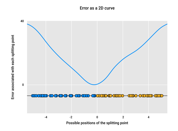
• we can separate the two classes using a single point on the line
• imagine sliding that point left and right:
  • each position gives us a different number of misclassified dots (the "error")
  • we can plot this error for each position giving us an error curve
• our goal is to find the minimum point on this error curve to get the best classifier
• for this particular dataset, the error is lowest (zero) when the dividing point is just to the left of 0

Adjusting the learning rate

Constant-sized updates

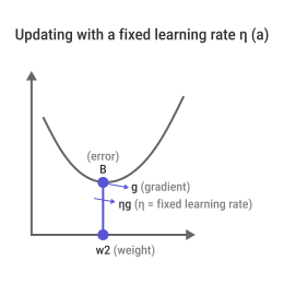
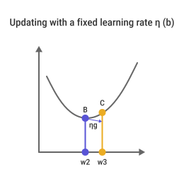
To update a weight using a constant learning rate (η, eta):

Step	Explanation	Image
Find the gradient	a weight w1 (not shown) was updated to value w2, and we want a better value w3 w2's error is point B find the gradient g at point B and scale it by the fixed learning rate → ηg ηg points in the same direction as g (smaller or same size) since 0 < η ≤ 1
Update the weight	add the scaled gradient ηg to w2 graphically, place the tail of the arrow ηg at B the tip of the arrow gives w3 w3's error is point C In this case, the step overshoots slightly and increases the error.

Instead of settling at the lowest point, the algorithm overshoots repeatedly:

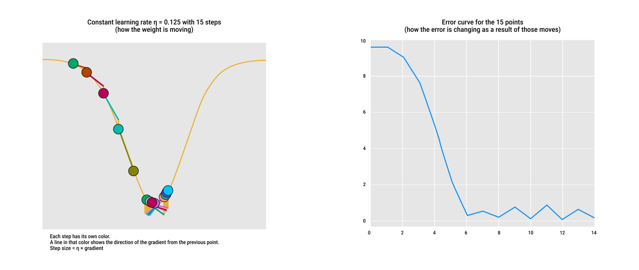
• a large learning rate is used (η ≈ 1/8 or 0.125) to better illustrate the steps (smaller rates behave similarly but more slowly)
• step size = η × gradient:
  • at the top of the curve, gradients are small, so steps are small
  • as the slope increases, steps get larger
• when we reach the bottom, the weight oscillates around the minimum because steps remain too large

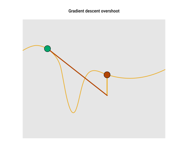
Missing a valley is a possible consequence of a large learning rate:

Changing the learning rate over time

A better approach is to adapt the learning rate over time with:

• large η at the start to avoid slow learning
• smaller η later to prevent bouncing around the minimum

This can be done by multiplying η by a decay parameter (slightly less than 1) at each update:

• start with η = 0.1 and decay = 0.99
• after step 1: η = 0.1 x 0.99 = 0.099
• after step 2: η = 0.099 x 0.99 = 0.09801
• and so on… over time, η decreases smoothly

Visualization of the value of η across many steps with various multipliers:

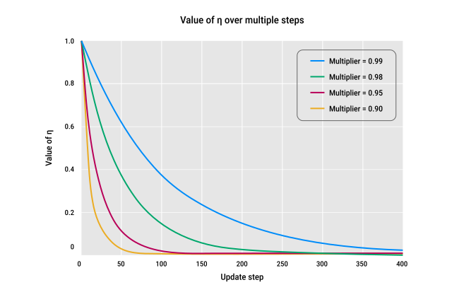
Writing this as an equation naturally involves exponents, so this kind of decreasing curve is called an exponential decay curve.

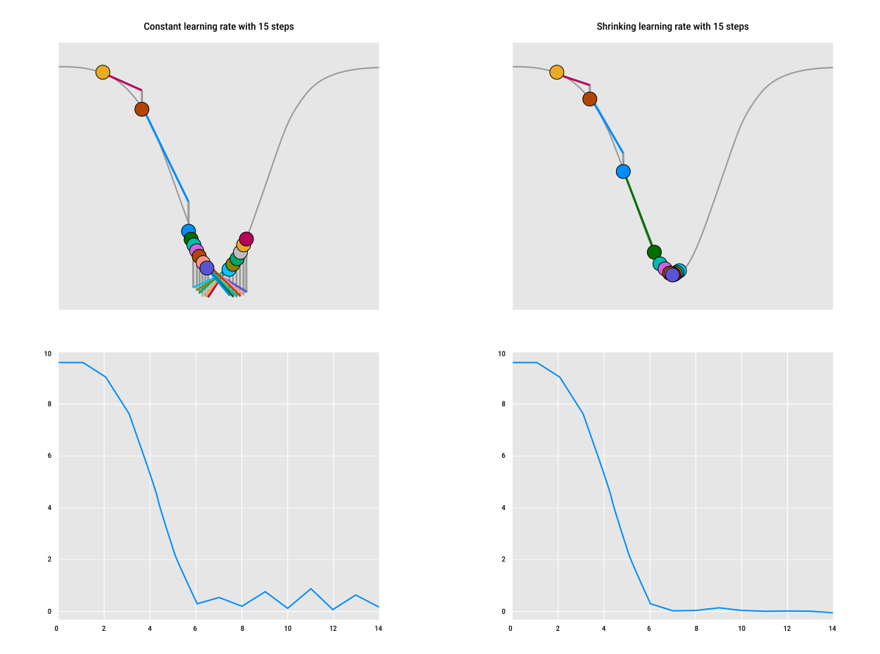
Compared to a constant learning rate, exponential decay efficiently settles the model into the lowest point of the error curve:

Decay schedules

Using a decay introduces two main challenges:

1. choosing the right value for the decay parameter
2. deciding when to apply decay (not necessarily after every update)

Strategies for adjusting the learning rate over time are called decay schedules, usually applied per epoch.

Common decay scheduling methods:

Name	Description	Image
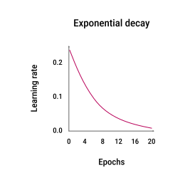
Exponential decay	Reduce the learning rate after every epoch.
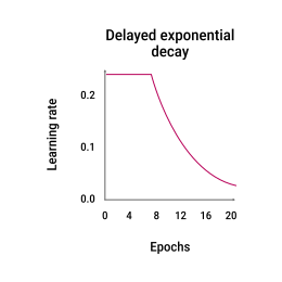
Delayed exponential decay	Wait a few epochs before starting decay so weights can move away from random initialization.
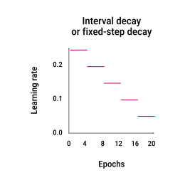
Interval decay (or fixed-step decay)	Reduce the learning rate every fixed number of epochs (e.g., every 4 or 10) to avoid shrinking too fast.
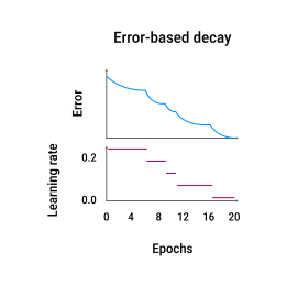
Error-based decay	Keep the learning rate while error decreases; apply decay when the network stops improving.

This raises natural questions:

• can learning rates be adjusted automatically without a preset schedule?
• can each weight have its own optimal learning rate?

Some gradient descent variations address these ideas.

Improving gradient descent

Different algorithms can improve gradient descent.

We compare the performance of three of them using the same setup:

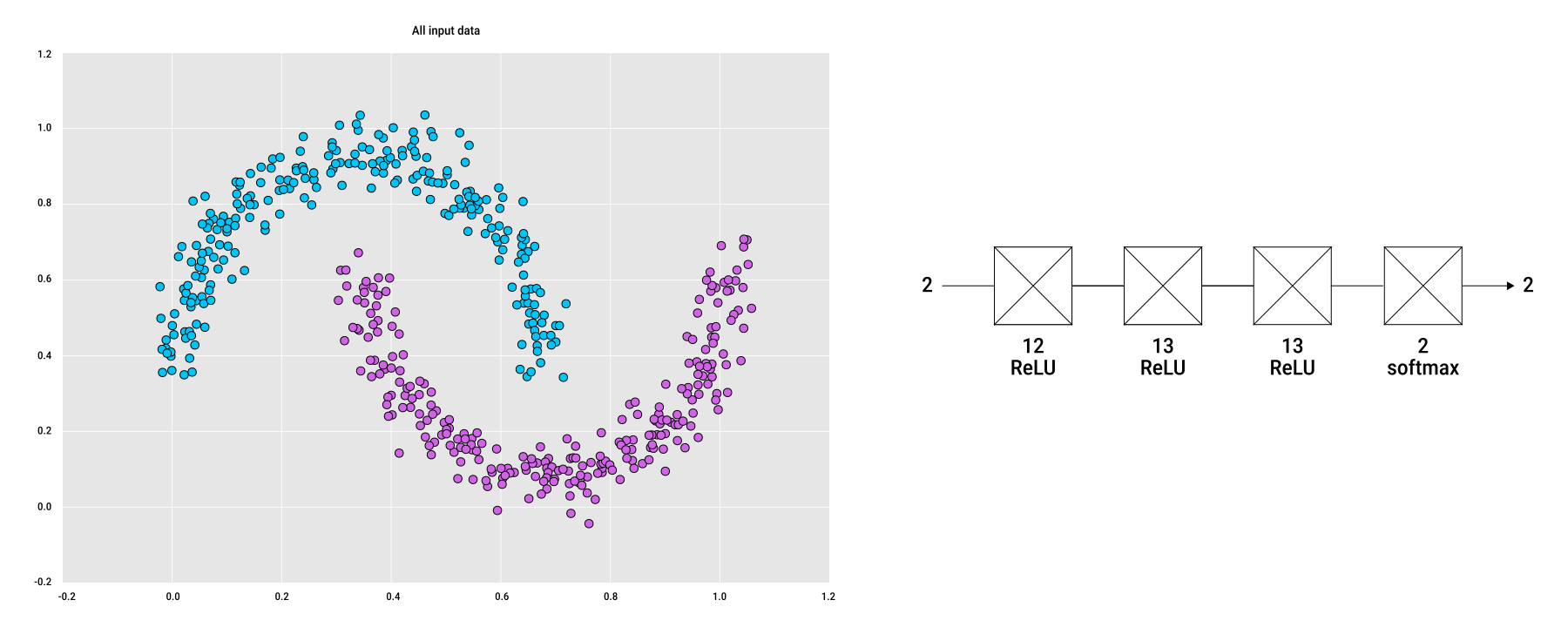
• dataset: 300 samples forming two fuzzy crescent-shaped classes of 150 points each
• neural network architecture:
  • 3 fully connected hidden layers (12, 13, 13 nodes), each using ReLU activation
  • 1 output layer with 2 nodes using softmax activation (class with higher probability is predicted)
• learning rate: a fixed rate of η = 0.01 is used for all experiments

Because each algorithm behaves differently, the number of epochs varies. Performance is compared after each epoch.

Feature	Batch gradient descent (BGD)	Stochastic gradient descent (SGD)	Mini-batch gradient descent
Notes	Also called epoch gradient descent	"Stochastic" (roughly "random") reflects that the network sees samples in a random order	The mini-batch is a fixed number of samples considerably smaller than the number of samples in the training set (usually a power of 2 between 32-256), chosen to fully utilize GPU parallelism
Gradient computation	Average of gradients over entire dataset	Gradient from one sample at a time (300 training samples = 300 updates per epoch)	Average of gradients over mini-batch of samples
Weights and biases update frequency	Once per epoch, after computing gradients for all samples in the dataset	After computing the gradient of every single sample	After each mini-batch, using the average gradient from that mini-batch
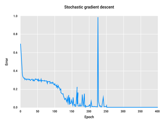
Performance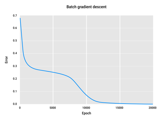
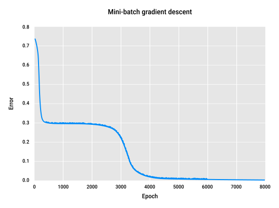Error curve	Very smooth (as it averages over all samples)	Fluctuates a lot (because we update after every sample and each one pulls weights in a different direction)	Moderately smooth, some noise
Epochs to converge	~20,000	~400	~5,000
Total weight updates	20,000 epochs × 1 update/epoch = 20,000	300 samples × 400 epochs = 120,000	300 samples, mini-batch size = 32 → number of mini-batches per epoch ≈ 300 ÷ 32 ≈ 10 → 10 * 5000 epochs = 50,000
Memory requirement	High (all data must be stored in memory)	Low (process samples one at a time)	Medium (store only mini-batches)
Advantages	Predictable, smooth learning; works offline (all data stored)	Faster convergence; does not require all data to be stored in memory	Compromise between BGD and SGD; efficient gains by using the GPU parallelism
Disadvantages	Slow for large datasets; requires storing all samples	Noisy error curve → hard to detect overfitting; can overshoot minima; more updates ≠ fewer epochs → total training time depends on number of updates (not just epochs)	Slight noise; still requires multiple updates; mini-batch size affects performance
Usage	Rare	Sometimes	Most common; often what is meant by "SGD" or "gradient descent" in literature

From this point forward, we'll refer to mini-batch gradient descent simply as SGD.

Gradient descent variations

SGD works well, but it has two key challenges:

1. choosing the right learning rate
2. dealing with flat or tricky regions of the loss surface (like saddles and plateaus)
   • research has shown that deep networks commonly have many saddles in their error landscapes:
   • systems need strategies to avoid or escape these regions

Gradient descent variations that address these issues:

• Momentum: helps roll over plateaus
• Nesterov: looks ahead for smoother steps
• AdaGrad: per-weight adaptive rate, but can vanish
• Adadelta/RMSprop: fixes vanishing updates
• Adam: combines momentum + RMSprop for fastest convergence

Momentum

Imagine the error surface as a 3D landscape:

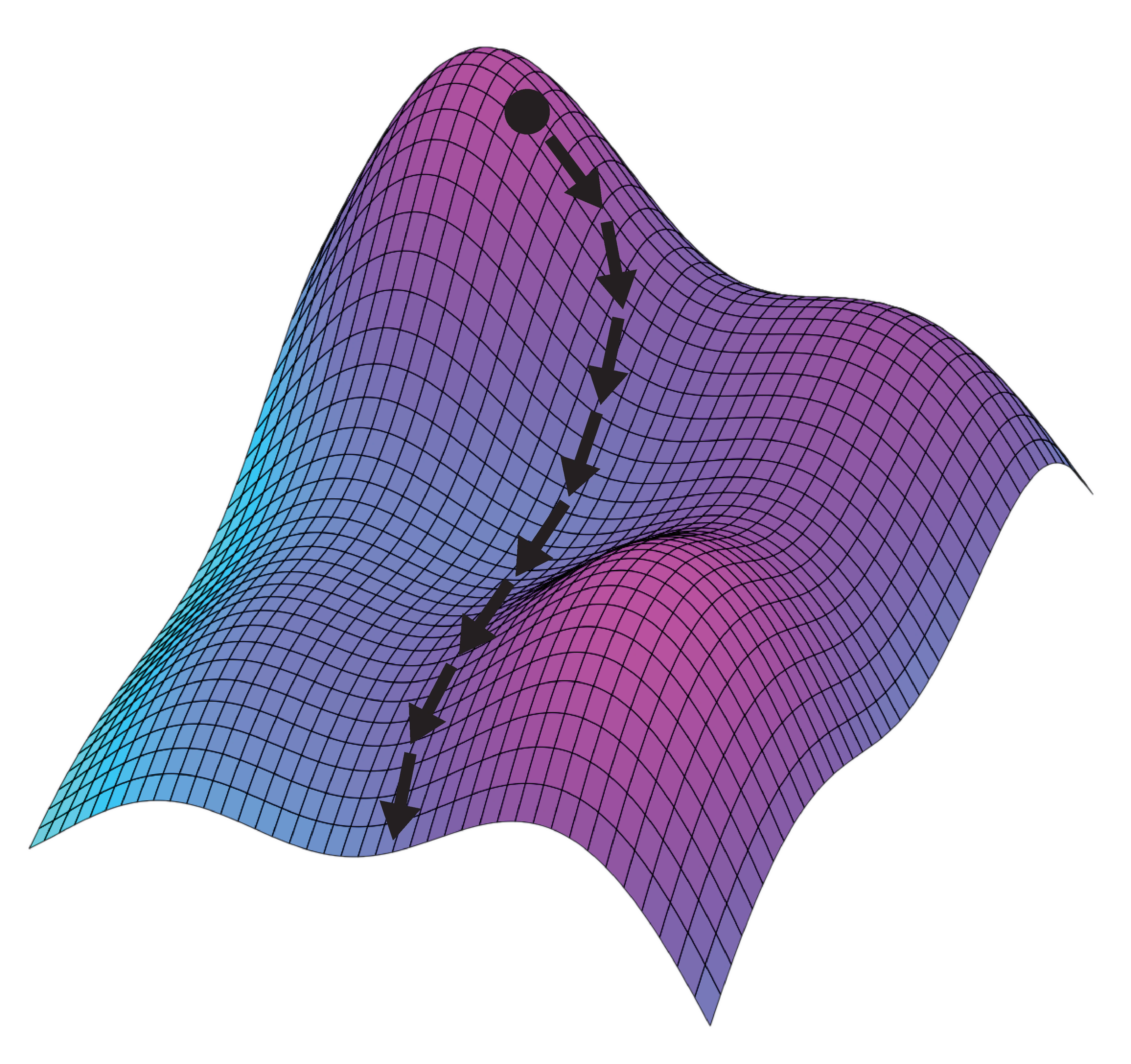
• the weights are plotted on the XY plane
• the height (Z-axis) shows the error of the weights
• a ball rolling downhill represents the model trying to minimize error by reaching the lowest point

A real rolling ball has inertia, which describes its resistance to a change in its motion.

A related idea is the ball's momentum or what keeps the ball moving across a plateau:

• without momentum: the ball slows and stops on flat regions
• with momentum: the ball keeps rolling across the plateau carrying some speed (inertia) that helps it reach the next valley

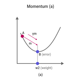
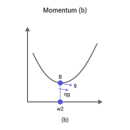
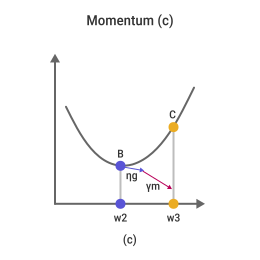
Momentum gradient descent adds inertia to gradient descent, combining the previous motion with the current gradient.

Finding the step for gradient descent with momentum:

Step	Explanation	Image
Find the previous motion	a weight w1 (not shown) with error A was updated to value w2 with error B, and we want a better value w3 with error C the previous motion (from A to B) is the momentum vector m scale it by the momentum scaling factor γ (gamma, 0 < γ ≤ 1), giving us γm
Gradient step	compute the gradient at B scale it by the learning rate η, giving us ηg
Combined update	add γm + ηg to B this gives the final direction and size of the next update graphically, place the tail of γm at the head of ηg

Momentum accelerates learning and helps escape plateaus and shallow minima.

Choosing the right momentum factor γ requires experience, intuition, and often trial and error. A common choice is γ ≈ 0.9.

Nesterov momentum

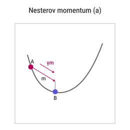
Instead of only calculating the gradient at the current position, Nesterov momentum:

• looks ahead to where we expect to be in the next step
• calculates the gradient at that future point
• uses that gradient to decide the next move

If the estimated future step:

• points in the same direction as before → we take a bigger step
• points in the opposite direction → we take a smaller step

Step	Explanation	Image
Start	the weight at position A is updated and ends up at B the motion from A to B becomes the momentum vector (the arrow m) it is scaled by γ (gamma) to get γm
Look ahead	instead of calculating the gradient at B add the scaled momentum to B to get the "predicted" error P this is where we think we're heading next on the error surface
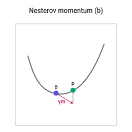
Find the gradient g at point P	compute the gradient g at point P scale it by the learning rate η (eta) → gives us ηg
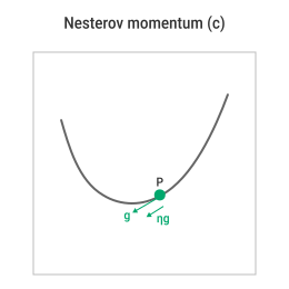
Update the position	add the scaled momentum γm and the scaled gradient ηg add both to B to get the next position C Notice that: we're not using the gradient at point B point C is closer to the bottom of the bowl than point P

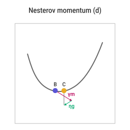
Compared to regular momentum, Nesterov momentum:

• uses no new parameters (still just γ and η)
• often leads to faster, smoother learning than regular momentum

AdaGrad

Adagrad (adaptive gradient learning) adapts the learning rate η on a per-weight basis.

For each weight, Adagrad:

1. takes the gradient from the current weight to update
2. squares it and adds it to a running sum for that weight
3. divides the original gradient by a value derived from this sum
4. uses that result to update the weight

A small initial learning rate, such as η = 0.01, often works well, with AdaGrad automatically handling adjustments over time.

Since gradients are squared, the sum is always positive and always grows.

To keep it from growing out of control:

• each change is divided by that growing sum
• as a result, the updates to each weight gradually decrease over time, eventually approaching zero and "vanishing"

Adadelta and RMSprop

These improved methods fix Adagrad's issue of endlessly shrinking updates.

Instead of summing all the squared gradients, Adadelta (adaptive delta) uses a decaying average of squared gradients (not full history), giving more weight to recent gradients and less to older ones:

• think of this as a running list of recent gradients for each weight
• each time we update the weights:
  • add the new gradient to the end of the list
  • delete the oldest one
• to find the value to use to divide the new gradient:
  • compute a weighted sum of the list
  • recent values get larger weights
  • oldest values get smaller weights

This creates a weighted average that is most heavily determined by recent gradients but also influenced to a lesser degree by the older gradients.

Adadelta requires additional hyperparameters:

• gamma γ (decay rate):
  • not to be confused with γ from momentum — it's a different concept!
  • controls how much we "remember" old gradients:
    • large γ = remembers older values more
    • small γ = focuses on recent gradients
  • common value 0.9
• epsilon ε (stability constant):
  • small value added to avoid division by zero
  • usually set automatically by libraries

RMSprop is similar to Adadelta, but uses slightly different math:

• RMS = Root Mean Square
• prop = propagation (referring to the backpropagation of gradients)

So the name literally describes: backpropagated gradients, scaled by the RMS of recent gradients.

Adam

For each weight, Adam (Adaptive Moment Estimation) keeps track of two running averages:

1. a moving average of the raw gradients
2. a moving average of the squared gradients

Previous algorithms used only squared gradients, which lost the sign information of the gradient.

Adam uses both lists to compute a more effective scaling factor.

Adam requires additional hyperparameters:

• β1 (beta 1): controls how much past gradients influence the current average
• β2 (beta 2): controls how much past squared gradients are remembered

Common default values: β1 = 0.9 and β2 = 0.999 (as per the original Adam paper).

Choosing an optimizer

Summary of the two-moon results for different algorithms:

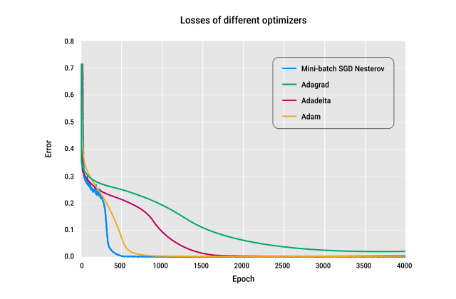
• in this simple case, mini-batch SGD with Nesterov momentum is the winner
• but in more complicated situations, adaptive optimizers (like Adam) often work better

Across many models and datasets:

• Adadelta, RMSprop and Adam often perform similarly
• Adam is a solid default — fast, stable, and works well out of the box

Why are there so many optimizers?

• because no single optimizer is best for every training problem
• the "best" optimizer depends on the data, model, and training setup
• most deep learning libraries offer routines that carry out an automated search and run through multiple parameters

Regularization

Even with the best optimizer, neural networks can overfit.

Regularization methods delay the onset of overfitting during training by:

• preventing individual neurons from producing huge outputs that dominate others
• spreading learning across the network

Dropout

Dropout is a regularization technique used during training:

• at the start of each training batch, a percentage of neurons (e.g., 20%) from the previous layer are randomly disabled
• once that batch is complete, the dropped neurons are restored

It is implemented as a dropout layer for conceptual clarity in network diagrams, but it's not a true layer:

• it has no neurons
• it performs no computation

Batchnorm

Batch normalization (or batchnorm) normalizes the outputs of the previous layer to a small range centered around 0:

• scaling and shifting parameters are learned during training (like weights)
• this may seem counterintuitive since training aims to produce useful outputs, but many activation functions (like ReLU or tanh) work best when inputs are near 0

It is implemented as a batchnorm layer:

• like dropout, it has no neurons
• unlike dropout, it does perform computation