Backpropagation

Backpropagation is the core algorithm used to train neural networks.

It works by adjusting the network's weights (initially random) to reduce error and produce the correct outputs.

To reduce error, we need to know whether each weight should be increased or decreased.

To figure that out, each neuron is given a delta value.

These delta values are calculated starting from the final output layer and moving backward to the first.

Because this process passes information backward through the layers, it's called backpropagation.

Backpropagation doesn't "propagate the error" but instead "propagates the gradient of the error".

Gradient descent

The gradient (or derivative) is the slope of the error curve at a particular weight.

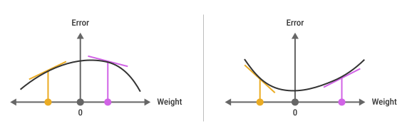
The sign of the gradient tells us the direction to move the weight to reduce error:

• positive (line goes up to the right): increasing the weight (moving it to the right) increases the error
• negative (line goes down to the right): increasing the weight reduces the error

The process of moving each weight in the direction that reduces error is named gradient descent because it uses the gradient to "descend" (reduce) the error.

By calculating gradients for all weights, we can update them simultaneously.

However, there's a challenge:

• changing one weight affects the output of its neuron
• this, in turn, affects all downstream neurons and their gradients
• as a result, some gradients may become outdated (e.g., a gradient that was positive may now be negative, and vice versa)

To manage this: small adjustments are made to each weight in the hopes that any such mistakes won't drown out improvements.

Backpropagation

For clarity, we ignore activation functions: they are essential in real networks, but here they only add extra detail.

Without activation functions, neurons only perform multiplication and addition. This leads to a key insight:

When a neuron's output changes, the final output error changes by a proportional amount.

A tiny neural network

Consider a tiny network (4 neurons, 8 weights) whose task is to classify 2D points into two categories (class 1 and class 2).

A single output neuron could handle two classes, but a larger network is used to demonstrate backpropagation principles:

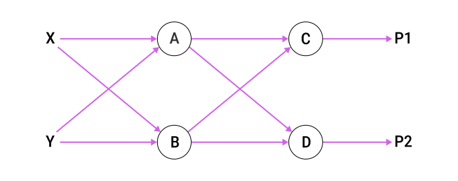
Conventions	Explanation
Ao, Bo, etc.	Output of neuron A, B, etc.
Aδ, Bδ, etc.	Delta value for neuron A, B, etc.
P1, P2	Predictions made by the network. Note: P1 = Co and P2 = Do.
Am	A change in the output of neuron A due to a change by an amount m.
E	The network's total error.
Em	Change in the error.

Output neurons

Backpropagation starts at the end of the network.

The output layer is a special case because there is no next layer.

So gradients come directly from the network error.

Calculating the network error

To obtain a single number representing the network's error:

• compare labels and predictions which are one-hot encoded:
  • (1, 0) → true label for a sample in class 1
  • (0, 1) → true label for a sample in class 2
  • (P1, P2) → network predictions
• example of prediction for a class 1 sample:
  • (P1, P2) = (1.0, 0.0) → ideal prediction
  • (P1, P2) = (0.8, 0.2) → less confident prediction

The difference between prediction and label is measured using cross-entropy:

Network Error = CrossEntropy( (P1, P2), TrueLabel )

Deep learning libraries provide this function, which returns both the error and its gradient:

• the error quantifies how far the predictions are from the true labels
• the gradient shows how the error will change

From gradient to delta

We can't see the full error curve for a neuron's output, but we can calculate its slope at any point:

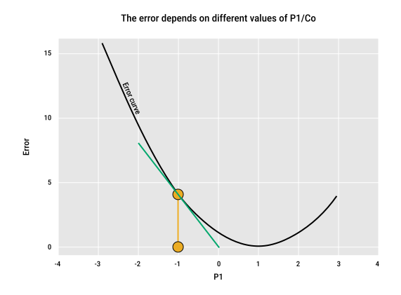
• the full error curve of P1 isn't given by the math
• instead, we can calculate the slope at any point, which is the derivative or gradient (shown as the green line)
• this slope shows which direction to move to reduce the error, as long as the steps are small enough to keep us close enough to its value

The delta (δ or Δ) is the gradient evaluated at a specific neuron's output:

• it's a real number (positive or negative)
• it measures how sensitive the network's error is to a small change in a neuron's output

Finding deltas for P1 and P2

For P1:

• estimate Cδ (the slope of the green line):
  • left: (-2, 8), middle: (-1, 4), right: (0, 0)
  • thus a change of +1 in P1/Co results in a change of -4 in the error
  • Cδ = -4
• -4 tells how sensitive the error is to changes at that point:
• say we now increase Co by Cm = 1/4:
  • a positive step, though in practice steps should be small to keep the gradient prediction accurate
  • the error will change by Em = Cm x Cδ = 1/4 × -4 = -1 (amplified by Cδ)
  • new error = previous error + Em = 4 + (-1) = 3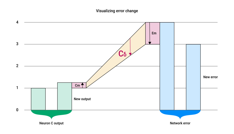
  • 

As soon as Co changes, the error curve changes too, so the derivative and Cδ must be recalculated.

The same process applies to find Dδ for P2.

The goal is to nudge all weights together until the error is as small as possible. Getting to exactly 0 error isn't always desirable, as continuing to train beyond a certain point can lead to overfitting.

Using deltas to change weights

Once we know the delta values for each neuron in the output layer, we can adjust the weights going into that layer.

Consider the weight AC:

• if we increase AC by 1:
  • old input to C = Ao × AC
  • new input to C = Ao × (AC + 1) = Ao × AC + Ao
  • → the input to C increases by exactly Ao
• therefore, the change in network error is proportional to Ao × Cδ

To reduce the error, we adjust the weight in the opposite direction:

• we decrease AC by 1
• → the network error decreases by Ao × Cδ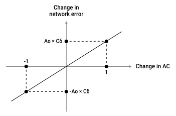
• 

This gives the weight update rule: AC = AC − (Ao × Cδ).

This rule applies to all weights feeding into the output layer.

Other neurons' deltas

Next, we compute deltas for neurons in the previous hidden layer.

If the output of a neuron (like neuron A) changes, that change affects the network error through every neuron it connects to in the next layer (neurons C and D in our example).

A change in A's output affects the error via C:

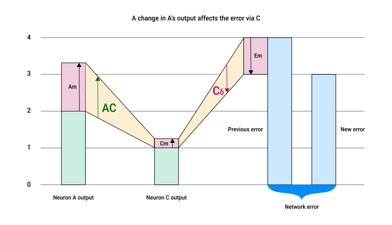
• Ao increases by an amount Am
• this change passes through the connection weight AC causing Co to change by Cm = Am x AC
• this change affects the total error and is measured by C's delta (Cδ)
• therefore:
  • change in the network error = Cm x Cδ
  • change in the network error = Am x AC x Cδ (substituting because Cm = Am x AC)
• from this, we can deduce A's delta (via C alone) : Aδ = AC x Cδ

Similarly, a change in A's output affects the error via D:

• we repeat the same reasoning: change in the network error = Am x AD x Dδ
• from this, we can deduce A's delta (via D alone) : Aδ = AD x Dδ

This means that a change in the output of neuron A influences the network's error through multiple paths at the same time:

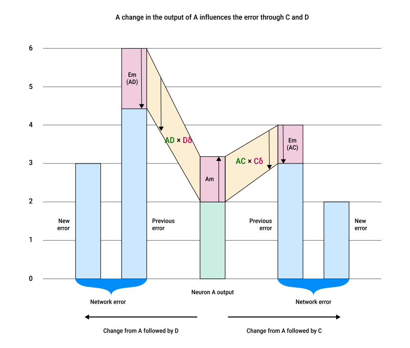
• each path produces its own change in the error:
  • one path goes A → C → Error
  • the other goes A → D → Error
• notice that neurons C and D have disappeared, only their deltas matter

Because neurons C and D do not affect each other, their contributions to the error are independent.

The total change to the error is just the sum of both contributions to the error:

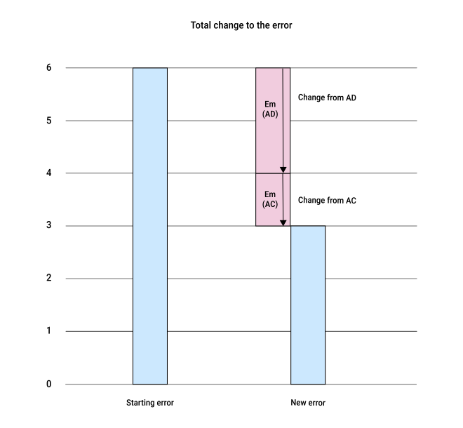
So the true delta for A must include both effects added together: Aδ = (AC x Cδ) + (AD x Dδ).

This is how to get the value of delta for any hidden neuron in any network:

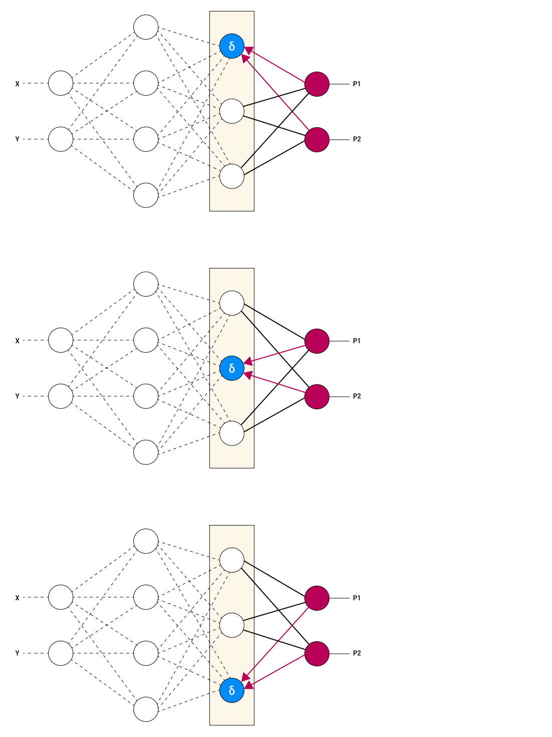
• multiply each next-layer delta by the weight connecting it
• sum all those results

Feed-forward and feed-backward are mirror processes

Deltas flow backward in the network, while outputs flow forward.

Example for any arbitrary neuron named H (we still ignore the activation function):

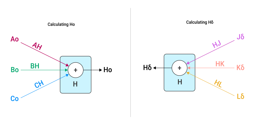
• left-to-right: compute output Ho with the values from the previous layer
  • multiply each previous neuron output by its connection weight
  • add up the results
• right-to-left: compute delta Hδ with deltas from the next layer
  • multiply each next-layer delta by its connection weight
  • add up the results

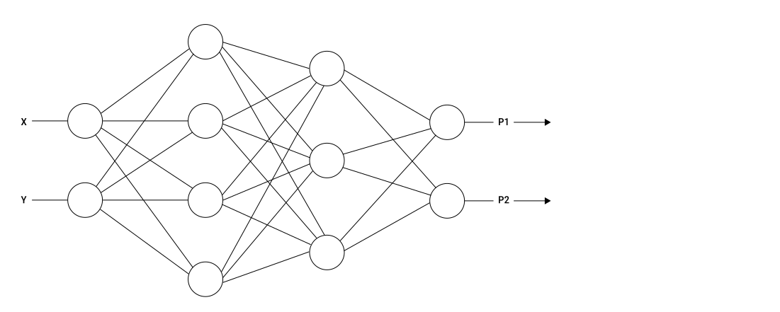
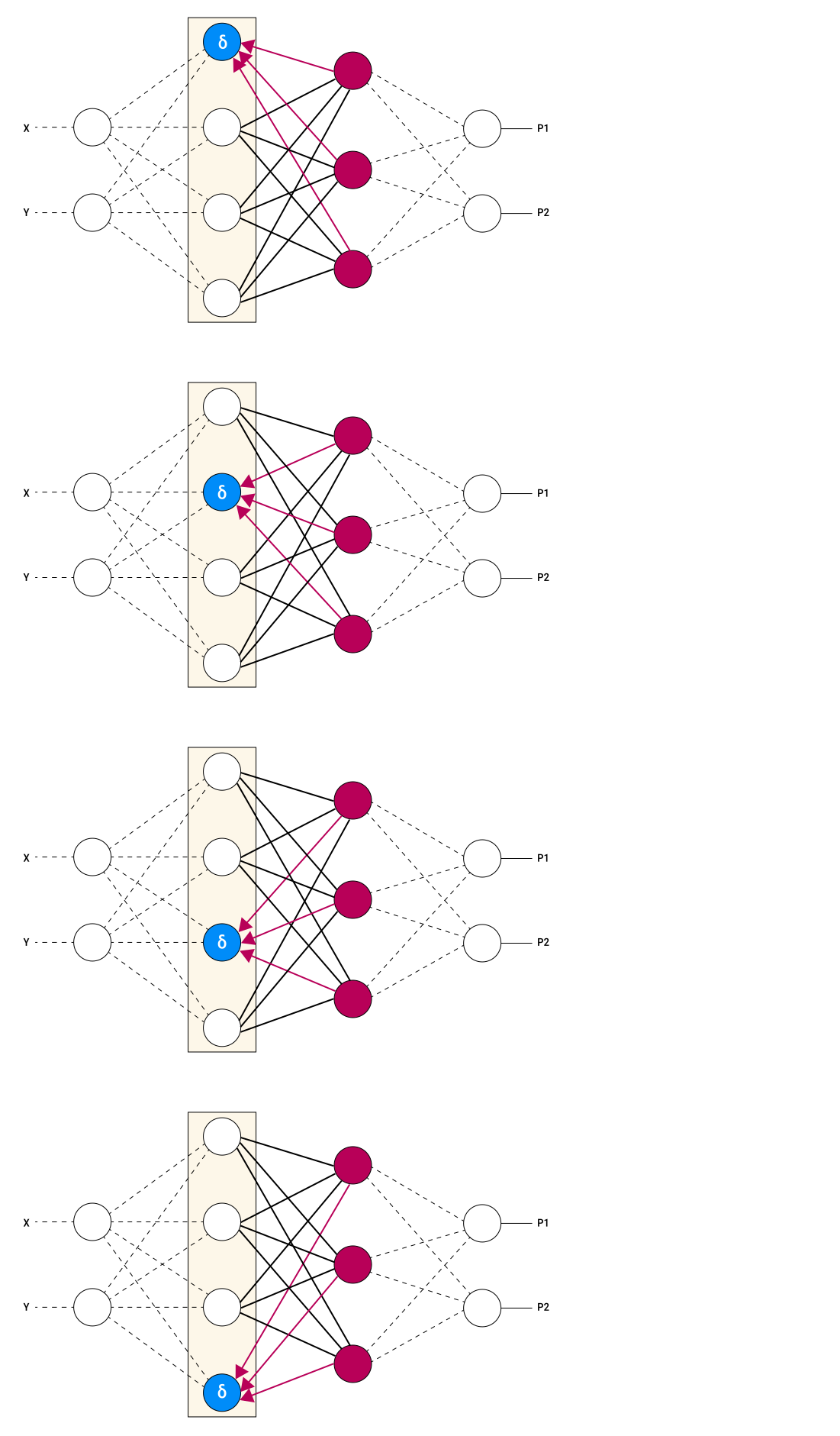
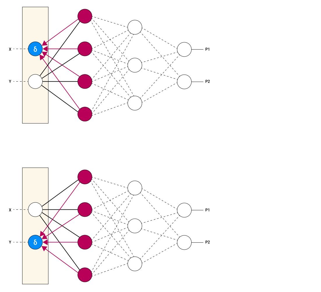
Backpropagation on a larger neural network

Step	Explanation	Image
Setup	Example network: 2 input neurons and 2 output neurons four layers three hidden layers (of 2, 4 and 3 neurons from left to right) Start by evaluating a sample: provide the values of its X and Y features to the input layer the network produces predictions: P1 and P2
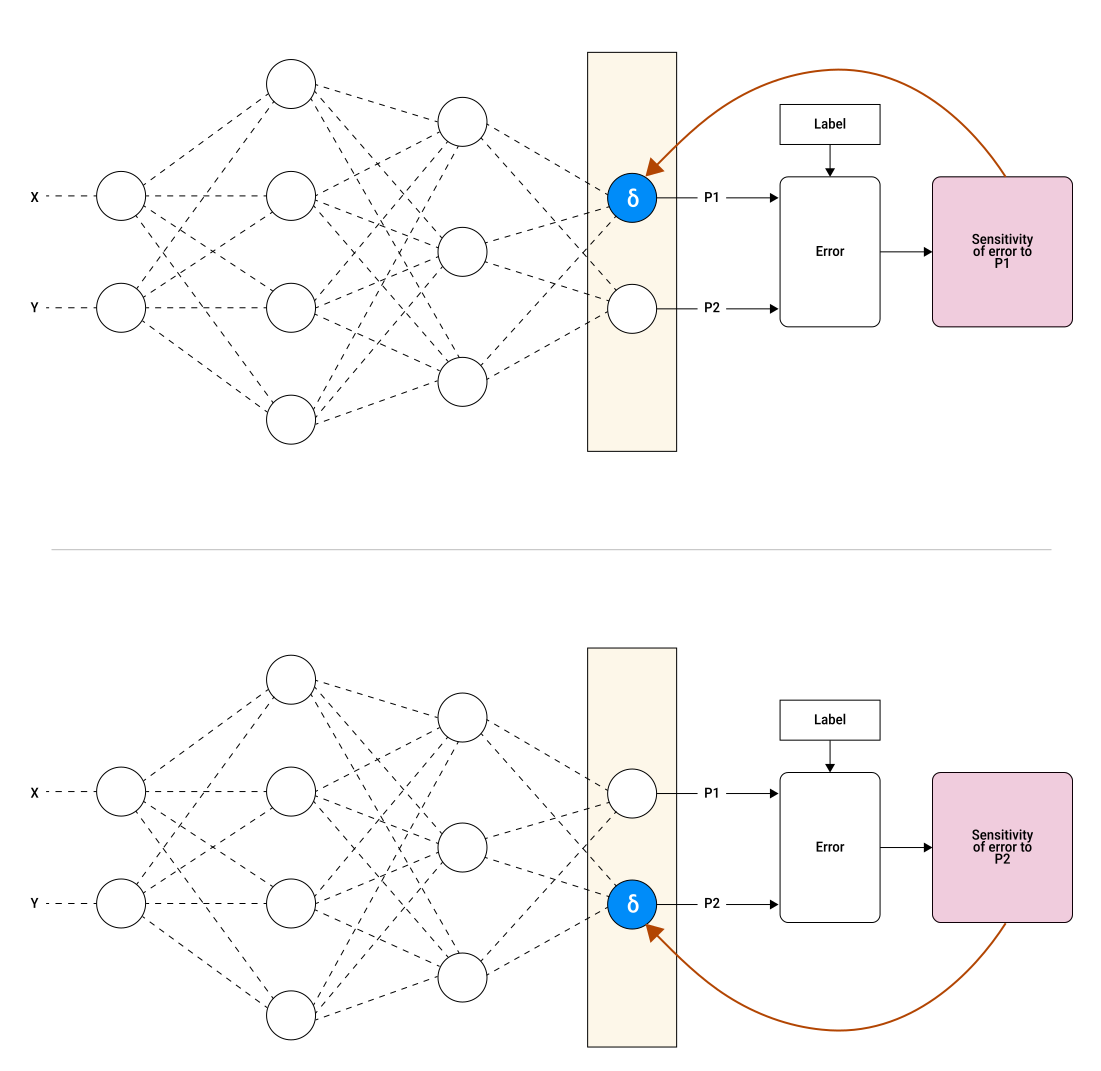
Compute deltas for the output layer	Compute the error for the output layer. Assume it's greater than zero (i.e., prediction isn't perfect). Compute the delta for the upper neuron (arbitrarily chosen) using a loss function (e.g., cross-entropy) and save it with the neuron. Repeat this process for all the other neurons in the output layer. At this point, every neuron in the output layer has a delta.
Compute deltas for the layer 3	Move one layer backward. For each neuron, compute its delta: find the deltas of all next-layer neurons that use its output multiply each by the connecting weight sum the results
Compute deltas for the layer 2	Move one layer backward. For each neuron, compute its delta: find the deltas of all next-layer neurons that use its output multiply each by the connecting weight sum the results
Compute deltas for the layer 1	Finally, move to the first hidden layer. For each neuron, compute its delta: find the deltas of all next-layer neurons that use its output multiply each by the connecting weight sum the results

Once all deltas are known, we can update the weights.

The final step is deciding how much to adjust each weight: a question answered by choosing the right learning rate.

The learning rate

Delta values indicate the direction in which weights should change to reduce error, but they are only accurate for tiny changes.

If weights change too much, the network may overshoot the minimum and become unstable; if too little, learning becomes slow.

The amount of changes to the weights is controlled by the learning rate (η, eta), a hyperparameter that scales weight changes:

• η = 0: weights never change, no learning
• η = 1: weights change a lot, errors may increase
• a common starting point is η = 0.001, then adjusting through trial and error

How the learning rate affects backpropagation?

Consider a simple binary classifier to separate the "two moons" dataset where about 1500 training data points are divided into two classes:

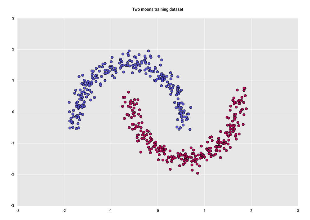
Classifier architecture:

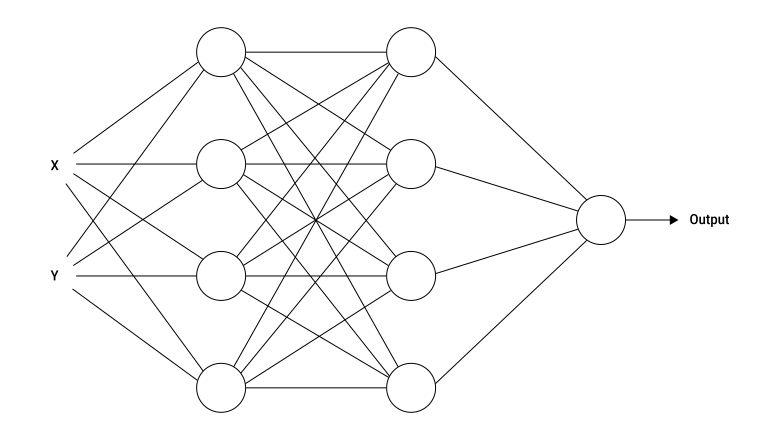
• two inputs
• 2 fully connected hidden layers, each with 4 neurons (using ReLU activation)
• one output layer (using sigmoid activation)
  • since we have only two classes, a binary classifier is all we need
  • the single output neuron interprets outputs near 0 as one class, and outputs near 1 as the other
• 28 connection weights + 9 bias terms = 37 weights

The goal is to adjust those 37 weights using backpropagation so the output matches the correct label.

Running backprop successfully relies on making small changes to the weights, but what counts as "small" depends on the network and the data.

We have to experiment with different learning rates to find out:

Learning rate	Explanation	Image
0.5 (large)	Decision boundaries are terrible: no clear decision boundaries everything is assigned to a single class (light background)
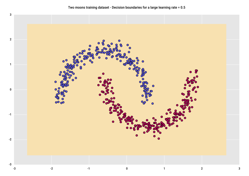
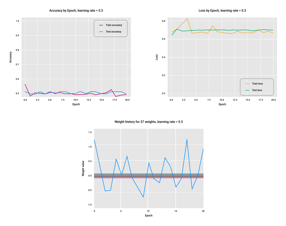
	Accuracy and loss: accuracy stays around 0.5, meaning half the data points are misclassified loss (or error) starts high and doesn't improve, even after many epochs Weights during training: one weight dominates the graph (it keeps overshooting its target) other weights are changing too little to make a visible difference These poor results aren't surprising because 0.5 is a very high learning rate and causes unstable updates.
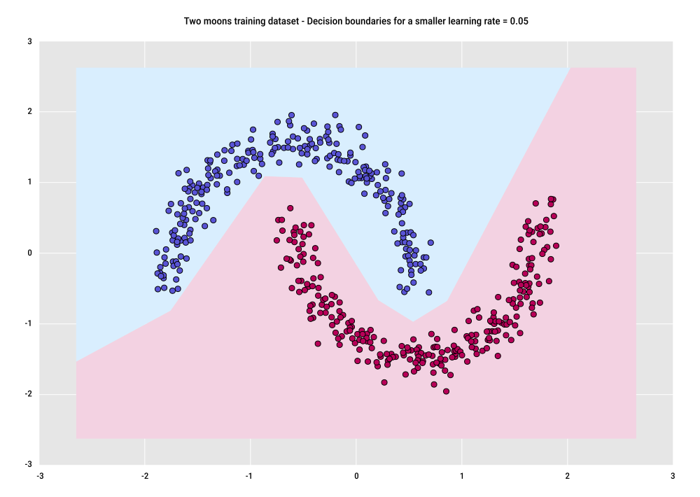
0.05 (reduce by a factor of 10)	Major improvement: clear and accurate class boundaries appear.
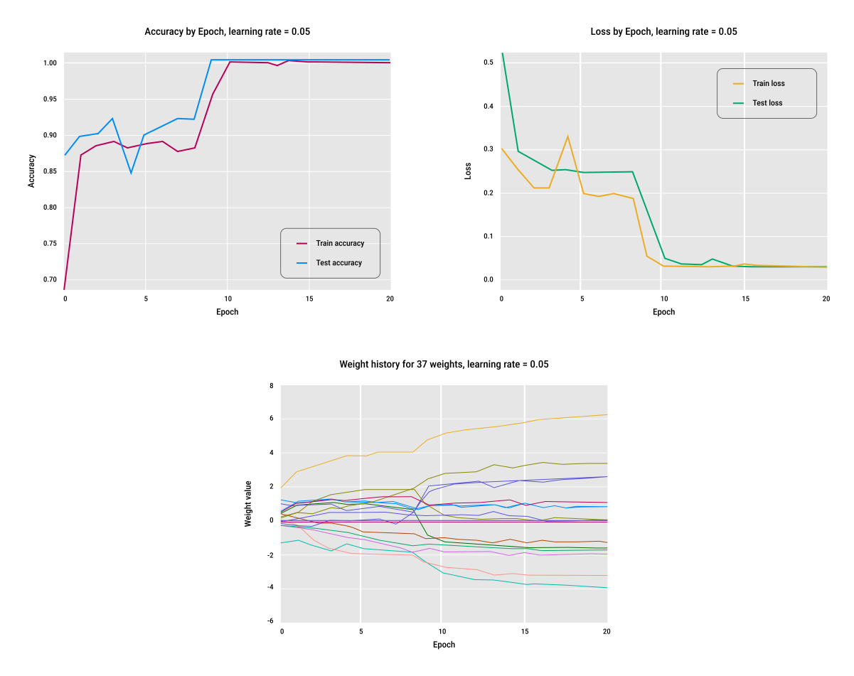
	Accuracy and loss: the network reaches 100% accuracy on both training and test sets after 10–16 epochs. Weights during training: many weights are now changing meaningfully some weights become quite large, which can slow or inhibit learning (ideally weights stay within a small range like [-1,1], this can be controlled with regularization) This setup works well: the network learns quickly and classifies the data perfectly.

Reducing the learning rate further to 0.01 has no real benefit here because the classification was already perfect at 0.05. For this network and this data, a smaller learning rate just makes training slower.

The learning rate must be tuned for each specific network and dataset (not too big, or too small, but just right).

If a network isn't learning, lowering the learning rate is often a good first step.

Algorithms can automatically adjust the learning rate in sophisticated ways.