Neural networks

Deep learning algorithms are built from networks of connected computational units called artificial neurons, which are inspired by the neurons in the human brain.

Neurons can be arranged into layers to form deep learning networks.

Biological neurons

A biological neuron:

• refers to a wide variety of complex cells distributed throughout every human body
• all neurons are similar in structure, but each type is specialized to perform different functions
• neurons communicate and perform their tasks using a mix of chemistry, physics, electricity, timing, proximity, and other biological mechanisms

A simplified biological neuron (shown in red below) sends its output to another neuron (in blue):

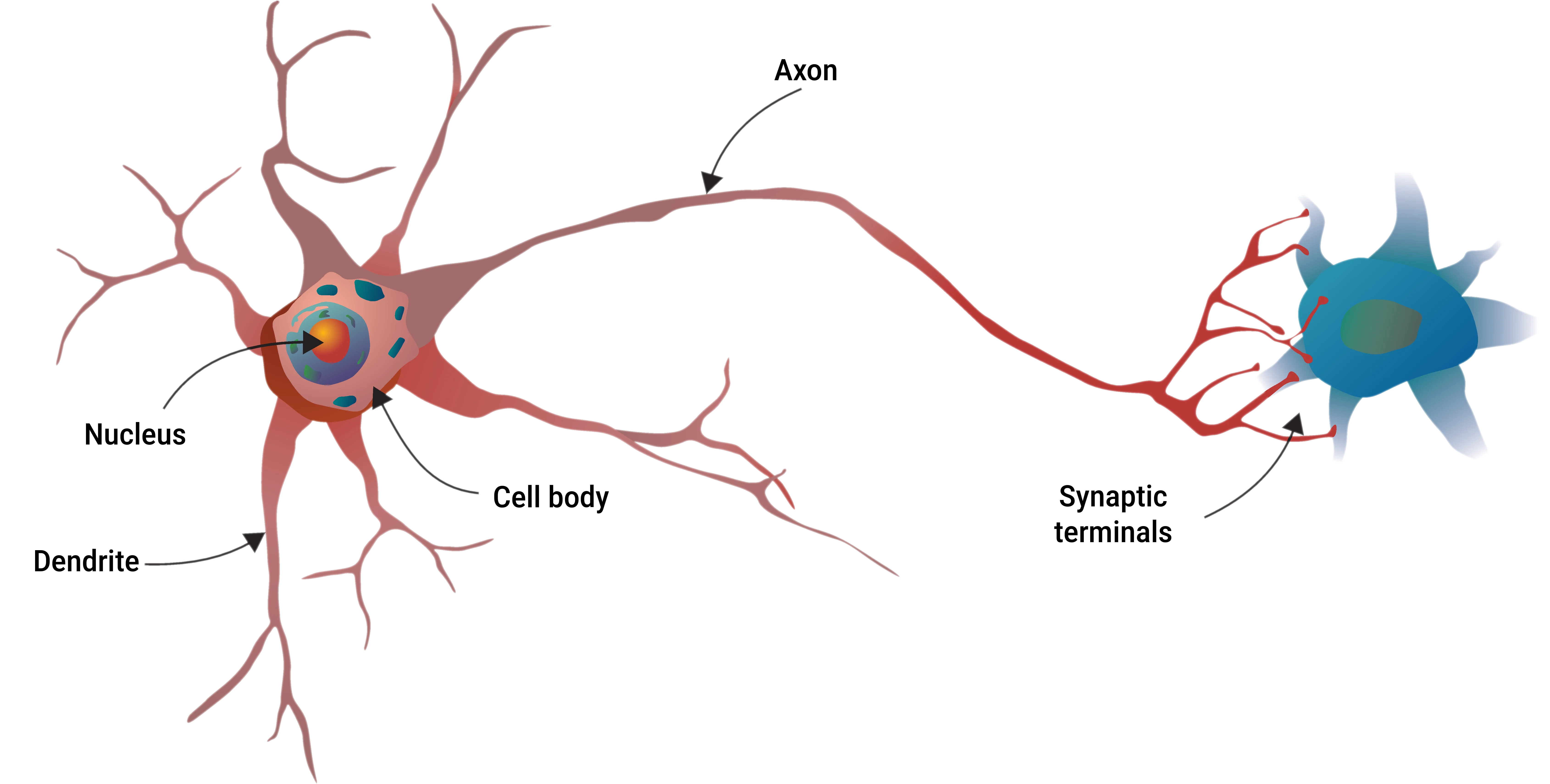
• biological neurons accept inputs on their dendrites
• when enough inputs are active, they "fire" to produce a short-lived voltage spike on their axons
• think of them as a light switch: off until there is a reason (sufficient input) to turn it on

Neuronal connections:

• two neurons are considered connected if one is physically close enough to receive signals released by the other, even without direct physical contact
• this pattern of connections is believed to be crucial to our thoughts, personality, and identity

Connectomes:

• a connectome is a map of an individual's neuronal connections
• connectomes are unique (comparable to fingerprints or iris patterns)

Scientists have tried to emulate the brain by creating large networks of simplified neurons in hardware or software.

So far, this has not produced human-like intelligence, but simplified neuron models can still solve many real-world problems effectively.

Artificial neurons

Artificial neurons in machine learning are basic versions of biological neurons.

They are improved versions of the original perceptron (1957).

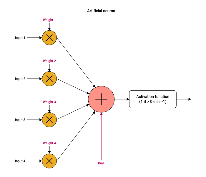
• every input to the neuron is multiplied by an associated weight
• an extra number called the bias is added to the sum of all the weighted inputs
• the neuron's output is calculated using an activation function:
  • called the activation function because the output of a real neuron is called its activation

Drawing the neurons

Diagrams are often simplified to stay clear and easy to read:

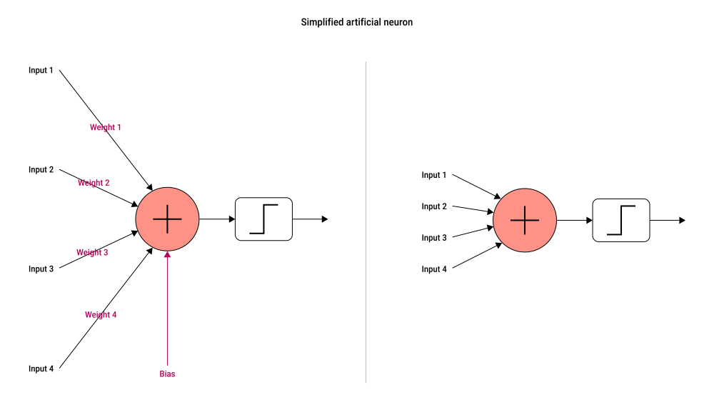
• weights and biases are hidden: we are expected to mentally include them
• the activation function is drawn with a small graphic of a function (a step function)

Even if not shown: biases and weights are always part of the neuron and are the only parameters that change during training.

Naming weights:

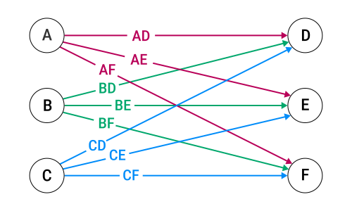
• sometimes, each neuron is labeled with a letter for convenience
• the weights are named by combining the letters of the connected neurons
• e.g., the weight from neuron A to neuron D is named AD

Feed-forward networks

In deep learning, neurons are arranged in layers:

• the neurons on each layer receive input only from the previous layer
• send their outputs only to the next layer
• do not communicate with other neurons on the same layer

The most common way to organize layers is the feed-forward network:

• earlier neurons feed values to later neurons
• data flows in one direction only

Neural network graphs

Neural networks are often shown as directed graphs:

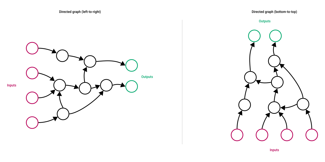
• a graph is made up of nodes (or vertices, elements) shown as circles
• nodes are connected by arrows called edges (or arcs, wires, lines)
• since information flows in only one direction, we call this a directed graph

How data flows:

• data enters through input nodes
• moves forward along the edges through the network
• is transformed at each node
• exits through output nodes

No loops or cycles:

• there are no loops or cycles
• this makes the graph a directed acyclic graph (DAG)
• the main exception is recurrent neural networks (RNNs), which allow feedback loops

Training and reverse flow (feed-backward):

• during training, a process called backpropagation sends error signals backward from outputs to inputs
• this temporarily reverses the flow of information to help adjust the weights

Initializing the weights

Training a neural network means adjusting its weights to improve performance.

How we initialize the weights helps the network learn faster and avoid issues like vanishing or exploding gradients during training.

Common initialization methods derived from theoretical research:

• LeCun Uniform, Glorot Uniform (or Xavier Uniform), He Uniform
  • select initial values from a uniform distribution
• LeCun Normal, Glorot Normal (or Xavier Normal), He Normal
  • select initial values from a normal distribution

Deep networks

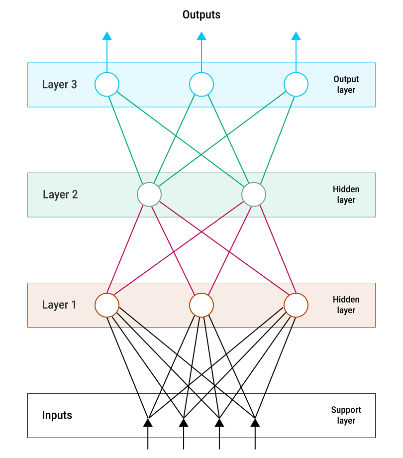
The phrase deep learning comes from stacking many layers vertically:

• the input layer is a support layer (no neurons) that holds raw data
• layers between the input and output are called hidden layers
• the output layer is the final one

The depth of a network is the number of layers that contain neurons (excluding the support layer).

Diagrams may show the data flow vertically or left-to-right.

A simple 3-layer network:

Fully connected layers

A fully connected layer (also called an FC, linear, or dense layer) connects every neuron to all neurons in the previous layer.

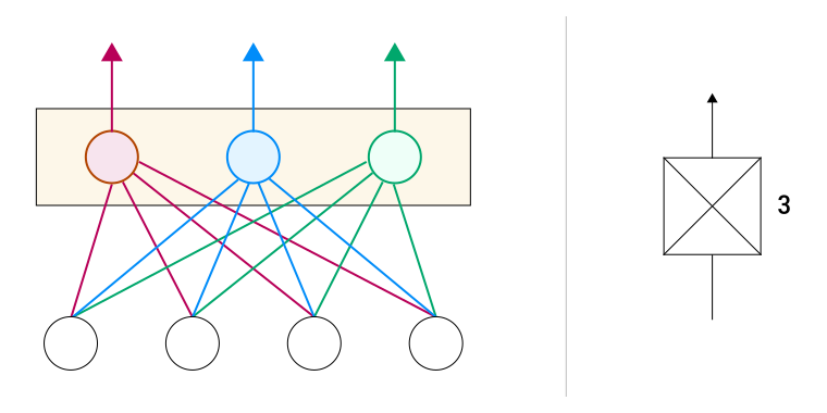
• left: the colored neurons make up a fully connected layer:
  • 3 neurons in the dense layer
  • 4 neurons in the preceding layer
  • 3 × 4 = 12 → total connections (each with a weight)
• right: icon for fully connected layers
  • next to the symbol, we identify how many neurons are in the layer (3 here)

Other layer types include convolutional and pooling layers, which organize neurons differently.

Tensors

Neural network layer outputs are often stored as arrays of numbers called tensors.

A tensor is a structured, multidimensional block of numbers with no gaps or extra elements.

Its shape is defined by the number of dimensions and the size of each.

Example of 1D, 2D, and 3D tensors represented as list, grid, and volume respectively:

Preventing network collapse

Activation functions are essential in neural networks.

Without activation functions:

• neurons only perform weighted sums (addition and multiplication), which are linear operations
• multiple layers of such neurons can be mathematically reduced to a single linear transformation
• as a result, the whole network remains linear and behaves like a single neuron

This phenomenon is called a network collapse: neurons can collapse (or combine) into a single neuron.

Activation functions prevent this by introducing nonlinearity, allowing the network to model more complex relationships.

Activation functions

An activation function takes a floating-point number as input and returns a new floating-point number as output.

It can be visualized as a graph:

• the input is on the horizontal (X) axis
• the output is on the vertical (Y) axis

Each neuron could use a different function, but in practice the same one is used for all neurons within a layer.

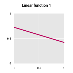
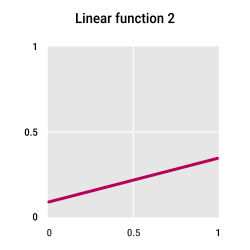
Straight-line functions

Straight-line functions are linear functions because they involve only addition and multiplication.

They can be represented as straight lines.

Linear functions can cause network collapse but are useful in two cases:

1. on output neurons: safe from collapse because no layers follow
2. as a processing step between the summation step in a neuron and its nonlinear activation function to pass values through without change

Name	Description	Image
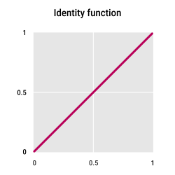
Identity function	The output always equals the input (y = x).
Linear function	Example 1.
Linear function	Example 2 tilted to a different slope.

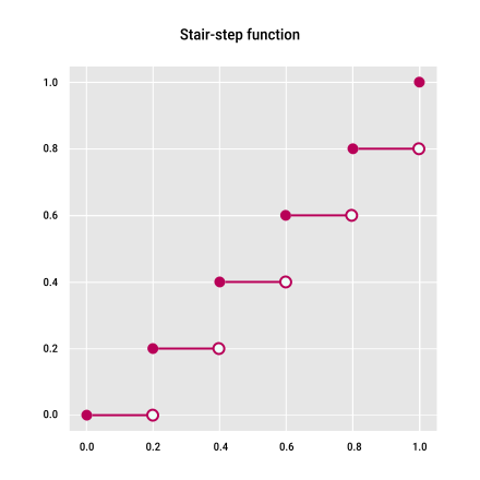
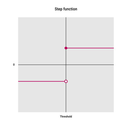
Step functions

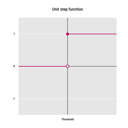
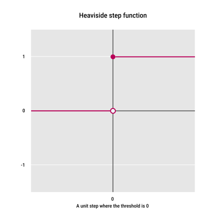
Step functions are a variation on linear functions.

Name	Description	Image
Stair-step function	The curve remains single-valued (each input x has only one output y). The output stays constant over intervals and then jumps to a new value at certain points. Here, a filled circle indicates that the y value is included.
Step function	One constant value on one side of the threshold and another value on the other side.
Unit step function	0 to the left of the threshold, 1 to the right.
Heaviside step function	A unit step where the threshold is 0. The "sign function" is a variation of this one where values to the left of 0 are -1 (rather than 0) and values to the right are 1. The original perceptron used a heaviside step function as its activation function.

Piecewise linear functions (ReLU)

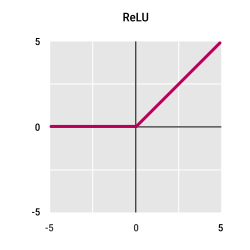
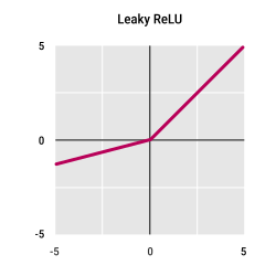
Piecewise linear functions are made up of multiple straight-line segments.

Name	Description	Image
ReLU	ReLU (e is lowercase) = Rectified Linear Unit. Named after electronic rectifiers that block negative voltage. A ReLU does the same for numbers: outputs 0 for negative inputs outputs the input itself for non-negative values Although it consists of two straight lines, the "bend" at 0 makes it nonlinear. Drawback: negative inputs always output 0, which can halt learning in a network. To address this, several ReLU variations have been developed.
Leaky ReLU	Outputs a small scaled-down value for negative inputs, instead of 0.
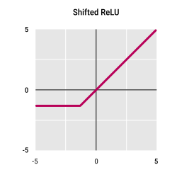
Shifted ReLU	Moves the bend of the ReLU function down and left.

Other variations:

• Parametric ReLU: similar to leaky ReLU, but the scaling factor for negative inputs is adjustable
• Maxout: a generalization that defines multiple lines and outputs the maximum value among them at each input, allowing more flexible shapes
• Noisy ReLU: adds a small random value to the input before applying a standard ReLU

Smooth functions (Sigmoid)

Training a neural network requires computing derivatives of each neuron's output, which necessarily involves their activation functions.

Earlier activation functions (like ReLU) are made of straight-line segments and have sharp corners where the derivative doesn't exist.

Even so, ReLU works because we can mathematically approximate the derivative at those corners, which is why ReLU remains popular.

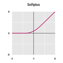
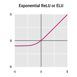
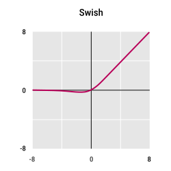
An alternative approach is to use smooth activation functions:

• they avoid sharp kinks and provide well-defined derivatives everywhere
• this makes them mathematically convenient for training neural networks while still introducing necessary nonlinearity

Example of smooth functions:

Name	Description	Image
Softplus	Smooth approximation of ReLU. Avoids the sharp bend at zero.
Exponential ReLU or ELU	Smooth version of Shifted ReLU. Allows negative output values.
Swish	Another way to smooth out the ReLU. Adds a small bump just left of 0. Transitions more gradually.
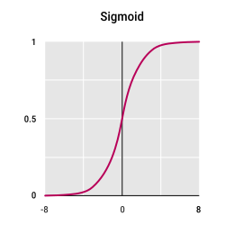
Sigmoid (or logistic function/curve)	Smooth version of the Heaviside Step. Output range [0, 1] (0 for very negative inputs, 1 for very positive). The name "sigmoid" comes from the resemblance of the curve to an "S" shape.
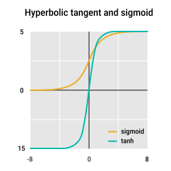
Hyperbolic tangent (tanh)	Similar to sigmoid but output range [-1, 1]. More centered around 0.
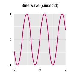
Sine wave	Output range: [-1, 1] (like tanh). Unlike tanh/sigmoid: it doesn't saturate (or stop changing) for inputs that are far from 0.

Comparing activation functions

There's no universal rule for choosing the best activation function.

It's based on experience and experimentation.

A few rules of thumb:

• use ReLU or leaky ReLU in hidden layers, especially fully connected ones
• for regression networks, use no activation (or a linear activation function) in the final layer to preserve exact output values
• for binary classification, use sigmoid in the final layer
• for multi-class classification, use a different activation function (e.g., softmax introduced next)

Softmax

Softmax is a function applied to the output layer of classification neural networks when there are two or more output neurons.

It converts raw output scores from the network into probabilities:

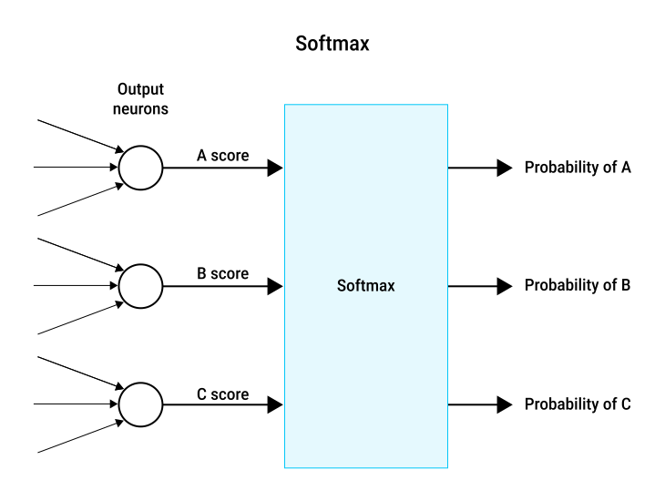
• softmax looks at all output scores together
• each score is converted into a probability for its class
• this allows for meaningful comparisons:
  • if one score is twice another, that does not mean the class is twice as likely
  • after softmax, if one probability is twice another, the class is truly twice as likely

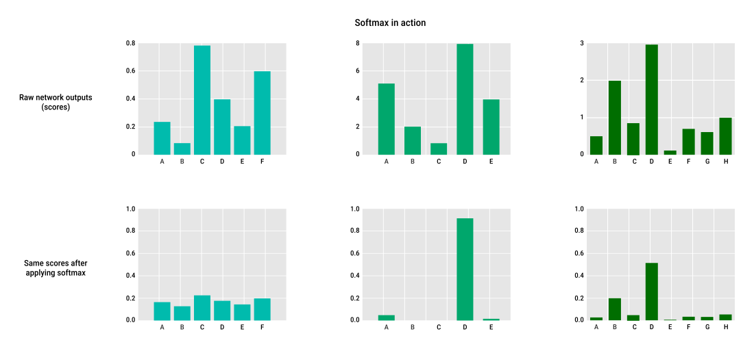
• note: the upper row uses different vertical scales
• left:
  • ranking of classes stays the same
  • large scores (e.g., C, F) are scaled down by a lot
  • smaller scores are scaled down only a little
• middle:
  • softmax exaggerates the largest value, making the prediction very confident
• right:
  • intermediate exaggeration