Bayes' rule

Frequentist and Bayesian probability

Two main approaches to probability:

• the frequentist approach searches for one correct answer
• the Bayesian approach (named after Thomas Bayes) searches for a range of likely outcomes (for example, predicting several possible next words in a text message rather than just one)

The Frequentist approach

A frequentist distrusts any specific measurements, treating them as approximations of a true value.

If a frequentist wants to know the height of a mountain:

• he combines a large number of observations
• the value that comes up most frequently is the one that's most probable

The Bayesian approach

A Bayesian trusts every measurement, though it may vary slightly.

If a Bayesian wants to know the height of a mountain:

• he says that the true value of the height of the mountain is a meaningless idea
• the height is a range of possibilities, each with its own probability
• as more measurements are taken, the range narrows but never collapses to a single number

Bayesian coin flipping

Consider a game with two coins:

1. one fair, with heads and tails equally likely
2. one rigged, with a bias of two-thirds, so it comes up heads two-thirds of the time

We pick a coin at random and want to figure out which one we got. It has a 50% chance of being fair and a 50% chance of being rigged.

What is the probability that the fair coin was picked?

We flip the coin once and observe Heads, so we can make a quantitative statement about which coin we picked.

Step	Explanation	Image
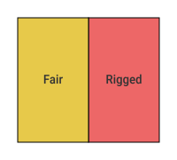
Picturing the coin probabilities	Represent the prior odds of choosing the fair coin (50:50) as a wall divided in half.
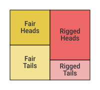
Split up the fair and rigged regions	Split each region by the probability of heads or tails. Now imagine throwing a dart at this wall. Wherever it lands represents the outcome of flipping a coin.
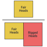
We've already flipped and observed heads	Since we've already flipped and observed heads, we know the dart must have landed in one of two zones: Fair Heads Rigged Heads The probability that the coin is fair given that we observed heads is the area of "Fair Heads" divided by the total area that produces heads. Because the "Rigged Heads" region is larger than the "Fair Heads" region: it's more likely that the observed Heads came from the rigged coin in other words, after seeing heads, we should update our belief: it's now slightly more likely that we flipped the rigged coin

Let's rephrase the last diagram using probability notation:

• P(H,F): probability of getting heads and the fair coin
• P(H,R): probability of getting heads and the rigged coin
• P(F|H): probability of getting the fair coin given that we observed heads

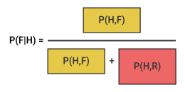
We can rewrite the joint probabilities by their expanded version:

\[\begin{aligned} \\ P(F|H) &= \frac{ {\color{Goldenrod}P(H,F)} }{ {\color{Goldenrod}P(H,F)} + {\color{crimson}P(H,R)} } \\ \\ &= \frac{ {\color{Goldenrod}P(H|F) \times P(F)} }{ {\color{Goldenrod}P(H|F) \times P(F)} + {\color{crimson}P(H|R) \times P(R)} } \\ \\ \end{aligned}\]

Let's assign a number to each term:

• P(F) = 1/2 → the probability that we picked the fair coin when we started
• P(R) = 1/2 → the probability that we picked the rigged coin when we started
• P(H|F) = 1/2 → the probability of getting heads given that we chose the fair coin
• P(H|R) = 2/3 → the probability of getting heads given that we chose the rigged coin

\[\begin{aligned} \\ P(F|H) &= \frac{ \frac{1}{2} \times \frac{1}{2} }{ (\frac{1}{2} \times \frac{1}{2}) + (\frac{2}{3} \times \frac{1}{2}) } \\ \\ &= \frac{ \frac{1}{4} }{ \frac{1}{4} + \frac{1}{3} } = \frac{ \frac{3}{12} }{ \frac{3}{12} + \frac{4}{12} } = \frac{3}{7} = 0.43 \\ \\ \end{aligned}\]

After just one flip:

• we can say that there's a 43% chance we picked the fair coin
• and therefore a 57% chance it's the rigged coin

Note:

• a frequentist wouldn't dare to characterize the coin as fair or not after just one flip
• but in the Bayesian view, we update our belief about which coin we likely have based on the observed result

Bayes' Rule

The bottom part of the ratio, P(H,F) + P(H,R) represents all the possible ways we could have gotten heads:

• it must come from either the fair coin or the rigged coin
• to simplify this:
  • we use a shortcut and replace the entire denominator with P(H) (the overall probability of getting heads)
  • without this shortcut, if we had 20 different coins, we'd need to sum 20 joint probabilities, which would make the expression very messy

\[\begin{aligned} \\ P(F|H) &= \frac{ P(H|F) \times P(F) }{ P(H,F) + P(H,R) } \\ \\ &= \frac{ P(H|F) \times P(F) }{ P(H) } \\ \\ \end{aligned}\]

This gives us the well-known Bayes' Rule (or Bayes' Theorem):

\[ \fbox{$ P(F|H) = \frac{ P(H|F) \ P(F)}{P(H)} $} \]

The left-hand side is always a conditional probability: "the probability of F given H". This is why the question we ask of Bayes' Rule needs to be in the form of a conditional probability:

What is the probability that (something1) is true, given that (something2) is true?

If we can't express our problem in that form, then Bayes' Rule isn't the right tool for answering it.

Bayes' Rule is tricky to remember, but it can be re-derived:

• write the joint probability of F and H in both forms:
  • P(F,H) and P(H,F)
  • these are the same thing: the probability of having a fair coin and getting heads
• replace them with their expanded versions
• divide each side by P(H)

\[\begin{aligned} \\ P(F,H) &= P(H,F)\\ \\ P(F|H) P(H) &= P(H|F) P(F)\\ \\ \frac{P(F|H) P(H)}{\relax{\color{ForestGreen}P(H)}\relax} &= \frac{P(H|F) P(F)}{\relax{\color{ForestGreen}P(H)}\relax}\\ \\ P(F|H) &= \frac{P(H|F) P(F)}{P(H)}\\ \\ \end{aligned}\]

Each term has a conventional name, and the traditional letters are A and B:

\[ \fbox{$ { {\color{BlueViolet}P(A|B)} \atop {\color{BlueViolet}\text{Posterior}\relax} } = \frac{ { {\color{crimson}\text{Likelihood}\relax} \atop {\color{crimson}P(B|A)} } \times { {\color{DarkOrchid}\text{Prior}\relax} \atop {\color{DarkOrchid}P(A)} } } { { {\color{ForestGreen}P(B)} \atop {\color{ForestGreen}\text{Evidence}\relax} } } $} \]

Term	Definition	Example
Prior P(A)	Belief about a hypothesis before observing data.	The chance the coin is fair before flipping it.
Likelihood P(B|A)	If the hypothesis were true, how likely would this observation be?	Getting heads if the coin is fair.
Evidence P(B)	The probability of the observed outcome.	Getting heads.
Posterior P(A|B)	The result of Bayes' Rule: the updated belief in the hypothesis after observing data.	The probability the coin is fair given that we saw heads.

A key strength of Bayesian reasoning is that it makes assumptions explicit through the prior P(A):

• it encodes our beliefs or expectations before we see any data
• it can be based on experience, previous data, or expert knowledge

While the likelihood P(B|A) and evidence P(B) usually come from the experimental setup, we have to guess the prior P(A).

In simple problems, such as a coin flip, choosing a prior is easy. In more complex settings, it is not.

Priors may be chosen by the analyst (subjective Bayes) or selected algorithmically (automatic Bayes).

Bayes' Rule and confusion matrices

Confusion matrices are useful when combined with Bayes' Rule to assess real-world probabilities.

Example:

• you're the captain of a spaceship
• your mission: find uninhabited planets to mine for raw materials
• the rule: never mine a planet that has life on it

So the question is:

Is there life on this planet?

To find out, you send a probe, which reports: "No life detected".

Because no probe is perfect, we must ask the question:

What is the probability that the planet contains life, given that the probe detected nothing?

Defining the events:

• L = Life is present = the ground truth
  • a positive value means the planet has life on it
• D = Detected life = the probe's result
  • a positive value means the probe detected life

The probe is sent to 1,000 known planets, of which 101 were known to contain life.

That gives us our prior:

• \( P(L) = 101/1,000 \) → about 10.1% of planets contain life
• out of every 1,000 planets we expect life on 101 of them

Probe testing results:

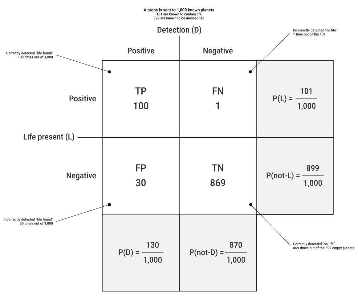
From the confusion matrix, we can compute:

• \( P(D) = 130/1,000 \)
• \( P(not-D) = 870/1,000 \)
• \( P(L) = 101/1,000 \)
• \( P(not-L) = 899/1,000 \)
• \( P(D|L) = 100/101 ≈ 0.99 \)
  • the recall TP / (TP + FN)
  • the probability that the probe reported life given that there really is life
• \( P(not-D|L) = 1/101 ≈ 0.01 \)
  • the false negative rate FN / (TP + FN)
  • the probability that the probe fails to detect life given that life is actually present

Using Bayes' Rule, \( P(L|not-D) \) is the probability that there actually is life given that our probe says there isn't:

\[\begin{aligned} \\ P(L|not-D) &= \frac{P(not-D|L) \times P(L)}{P(not-D)} \\ \\ &= \frac{ \frac{1}{101} \times \frac{101}{1,000} }{ \frac{870}{1,000} }\\ \\ &= \frac{ \frac{1}{1,000} }{ \frac{870}{1,000} } = \frac{1}{870} = 0.001 \\ \\ \end{aligned}\]

If the probe reports "no life", there's only a 0.1% chance the planet actually has life. That's a lot of confidence.

Now, what if the probe does detect life?

How confident can we be that there really is life on that planet?

\[\begin{aligned} \\ P(L|D) &= \frac{P(D|L) \times P(L)}{P(D)} \\ \\ &= \frac{ \frac{100}{101} \times \frac{101}{1,000} }{ \frac{130}{1,000} }\\ \\ &= \frac{ \frac{100}{1,000} }{ \frac{130}{1,000} } = \frac{100}{130} = 0.77 \\ \\ \end{aligned}\]

If the probe says it found life, we can be about 77% confident that life is truly there, just from this one probe.

To be even more sure:

• we can send down more probes to increase our confidence in either result
• but we'll never get to absolute certainty either way
• at some point we'll need to make a judgment call about whether to mine the planet or not

Repeating Bayes' rule

One event (or measurement) isn't much evidence.

If we apply Bayes' Rule repeatedly in a loop, we can refine our beliefs every time new data arrives.

Each round of Bayes' Rule works like this:

1. start with a prior P(A) or your initial belief
2. collect new evidence P(B)
3. apply Bayes' Rule to calculate the posterior P(A|B)
4. use this posterior as your new prior and repeat with the next piece of evidence

The Bayes Loop:

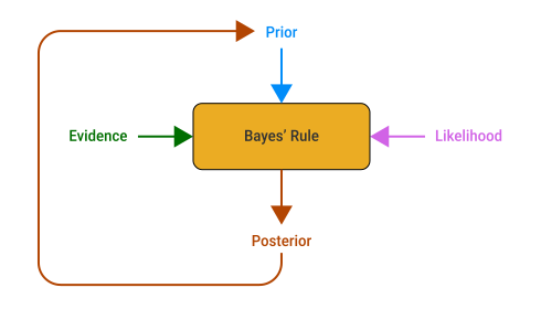
Each pass through the loop improves our prior, moving from a rough guess toward a more confident estimate.

Bayes' Rule accumulates evidence:

• as observations increase, confidence grows when data supports a hypothesis and declines when it contradicts it
• even small numbers of observations can give strong signals
• but absolute certainty is never reached — only high confidence
• the more observations you have, the more confidently you can distinguish between competing hypotheses

The Bayes Loop provides a systematic way to update our beliefs based on evidence, getting closer to the truth with each piece of new information.

Multiple hypotheses

Bayes' Rule can handle multiple hypotheses simultaneously — e.g., "the coin is fair" and "the coin is rigged".

Each hypothesis gets updated independently after every observation, allowing us to compare their relative probabilities.

Imagine a box containing coins with 5 different biases:

• each hypothesis corresponds to a different coin bias:
  • H0 bias = 0 (always tails)
  • H1 bias = 0.25 (25% heads, 75% tails)
  • H2 bias = 0.5 (fair coin)
  • H3 bias = 0.75 (75% heads, 25% tails)
  • H4 bias = 1 (always heads)
• we pick a coin at random and want to figure out which one we got
• each hypothesis has:
  • a prior — initial belief:
    • because we don't know anything about the coin we've selected:
      • each coin has equal probability or 1/5 = 0.2
      • so we assign equal priors (0.2 each)
    • we could get fancier but one of the beauties of the Bayesian approach is that:
      • we can start with almost any prior
      • that's even roughly close
      • and ultimately get the same results
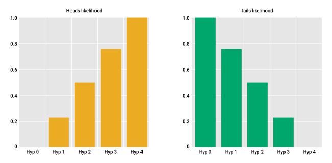
  • a likelihood — how likely the observed data is if that hypothesis were true
    • the likelihood for each hypothesis is simply the coin's bias
    • a coin with bias 0.25 has:
      • likelihood of coming up heads = 0.25 → 25% chance of heads
      • likelihood of coming up tails = 1 - 0.25 = 0.75 → 75% chance of tails
    • likelihoods are plotted in this figure:
      • 
    • these likelihoods stay constant throughout our experiment because the coins themselves don't change as we flip them and gather observations
  • a posterior (updated belief after seeing data)

After each coin flip, the posterior becomes the new prior for the next flip.

Result of the first flip → heads:

• 
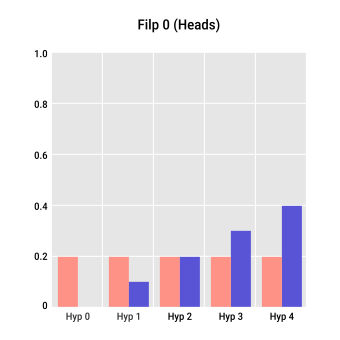
• all five hypotheses start with priors of 0.2 (pink bars)
• after seeing heads, we multiply each prior by its "heads" likelihood (yellow bars on the previous diagram)
• we get the posterior (blue bars - output of Bayes' Rule)
• H0 (bias = 0) drops to 0 because it predicts no heads
• H4 (bias = 1.0) rises the most since it always predicts heads
• after one flip, the "always heads" hypothesis looks best

The most likely hypothesis emerges gradually:

• as we keep flipping (say, 100 flips with ~30% heads), the probabilities shift gradually
• the system converges toward the hypothesis whose bias is closest to the true one
• in this case, it favors H1 (bias 0.25)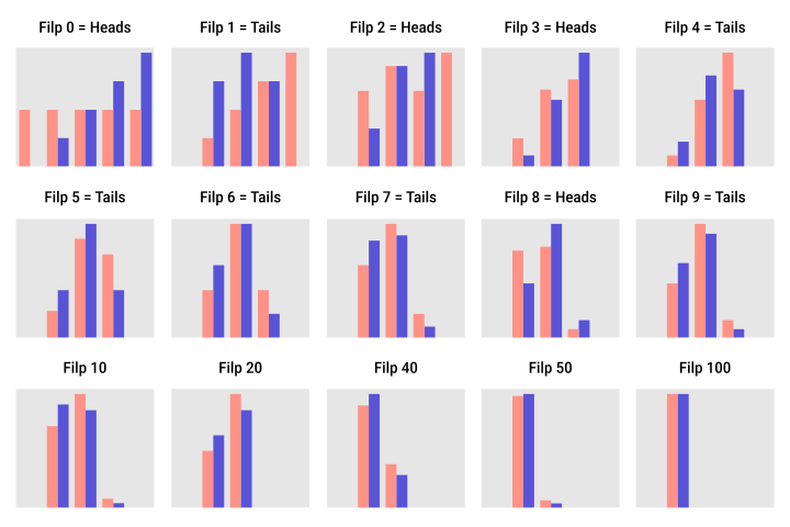
• 
• even if none of our hypotheses is an exact match, the system chooses the closest hypothesis

With many hypotheses, posteriors resemble a Gaussian curve:

• after 500 flips, the posterior distribution forms a Gaussian shape centered around the true bias (e.g., 0.3)
• the vertical bars are eliminated to better see the values of all 500 hypotheses
• 

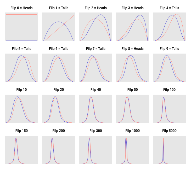
By increasing the number of hypotheses toward infinity, Bayesian updating naturally leads to continuous probability distributions, allowing arbitrarily precise estimates.

Robustness to poor priors:

• even with a wrong initial belief (e.g., prior centered at 0.8):
  • the system eventually converges on the correct bias (0.3)
  • though more slowly
• this shows Bayesian resilience:
  • even poor starting beliefs can lead to accurate conclusions with enough data