Measuring performance

We use performance metrics based on probability to evaluate a system.

Probability

Basic probability

We're throwing darts at the wall:

• every dart will strike the wall somewhere (not the floor or ceiling)
• the probability of hitting the wall somewhere is 1.0 (or a 100-percent chance)

Type	Description	Image
Simple probability P(A)	The chance of event A happening (e.g., hitting the red square): P(A) = red area ÷ total area Example: P(A) = 1/2 = 0.5 = 50%
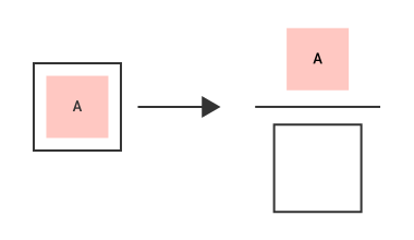
Conditional probability P(A|B)	The chance of A given that B happened: P(A|B) = overlap of A and B ÷ area of B (| means given) order matters: P(A|B) ≠ P(B|A), e.g., if 23 of 66 darts in B also land in A, P(A|B) ≈ 0.35, while P(B|A) ≈ 0.22
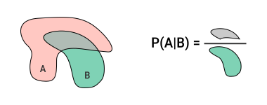
Joint probability P(A,B)	The chance of A and B happening together: P(A,B) = overlap of A and B ÷ total area order doesn't matter: P(A,B) = P(A|B) x P(B) = P(B|A) x P(A)
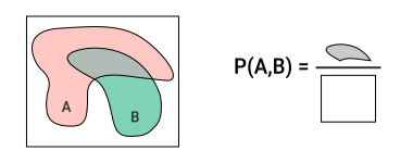
	Another way to look at the joint probability (useful with Bayes' Rule) using known probabilities: if P(B) and P(A|B) are known then P(A,B) = P(A|B) x P(B) this gives the probability of hitting both A and B at the same time Note: we're left with the gray area over the square because the green blobs of area B cancel each other.

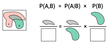
Marginal probability

Marginal probability is another term for simple probability.

The word marginal comes from books containing tables of precomputed probabilities written in the margin of the page.

Illustration with an ice cream shop example where customers are choosing between vanilla or chocolate and cup or waffle cone:

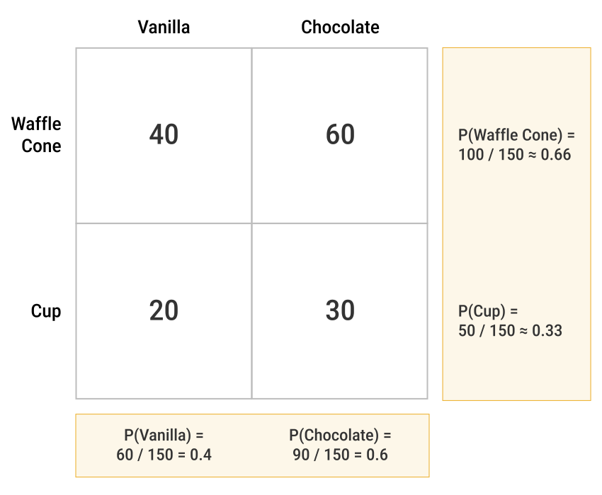
All the probabilities for the various outcomes of any event will always add up to 1 because it is 100 percent certain that one of the outcomes will occur.

Measuring correctness

We will work with systems that fall short of being perfectly accurate.

It's important to understand what kind of errors they make.

Binary classification

A binary classifier decides whether each data sample belongs to a class by answering a yes/no question:

• if "yes", the sample is called positive
• if "no", the sample is called negative

A classifier's performance is evaluated by comparing:

1. ground truth (also called manual label or actual value): the correct label assigned beforehand
2. predicted value: the label returned by the classifier

Perfect accuracy would mean "predictions = ground truth", but in practice, errors occur.

Classifier example:

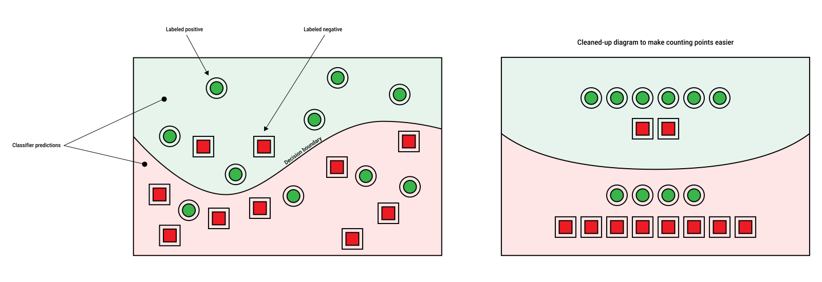
• each sample has two measurements (e.g., height and weight) plotted on a 2D grid
• ground truth labels are shown using color and shape:
  • positive → green circles
  • negative → red squares
• classifier predictions are shown by background color
  • positive → green background
  • negative → red background
• a decision boundary (curve) separates predicted positive and negative regions

Understanding errors is important:

• different types of mistakes can have different consequences
• knowing where and how a classifier fails helps decide whether it should be improved or replaced

The confusion matrix

A confusion matrix summarizes the results of a classifier, showing how many samples fell into one of four categories:

• True Positive (TP): correctly predicted positive
• True Negative (TN): correctly predicted negative
• False Positive (FP): incorrectly predicted positive
• False Negative (FN): incorrectly predicted negative

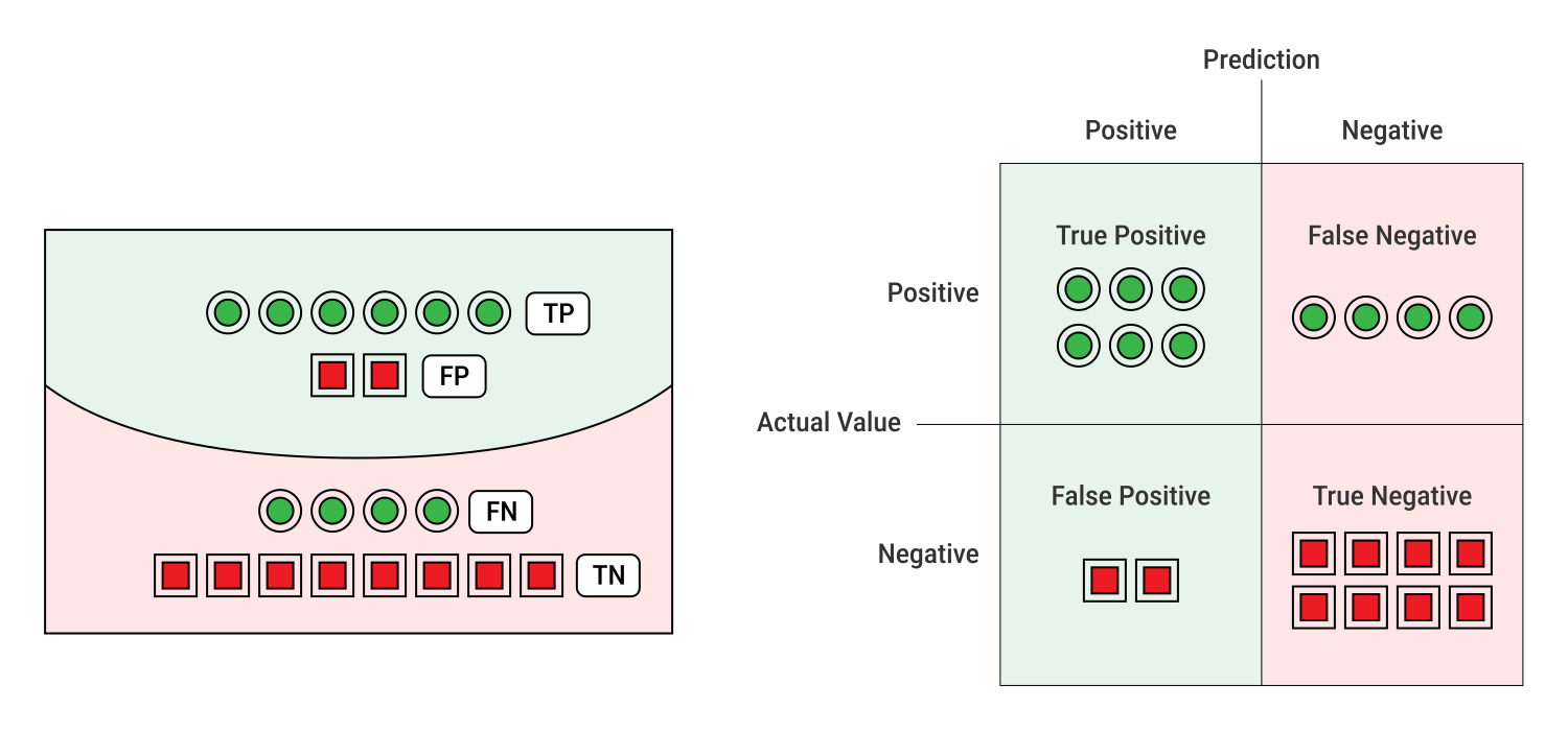
• 6 green circles correctly predicted as positive → TP
• 8 red squares correctly predicted as negative → TN
• 2 red squares incorrectly predicted as positive → FP
• 4 green circles incorrectly predicted as negative → FN

This can be written more concisely:

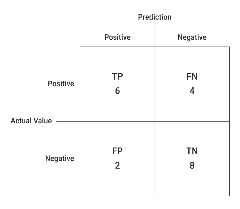
The confusion matrix as a table

	0	1	3	9
0	978	0	1	1
1	2	1,128	3	2
3	5	0	997	8
9	5	1	8	995

• rows: samples given to the model
• columns: model's responses
• when 0 was the input, the model was correct 978 out of 980 times
• when a classifier is good:
  • the numbers along the diagonal from upper left to lower right are high
  • there are almost no numbers off that diagonal (errors made by the model)

Measuring correct and incorrect

Looking at a confusion matrix can be, well, confusing.

We can characterize a binary classifier's performance using common statistics.

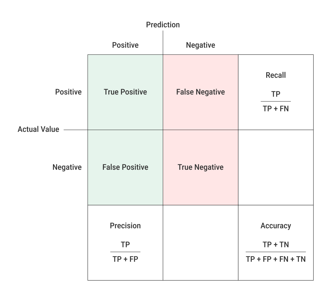
1. Accuracy or percentage of correctly predicted samples:

   • \( \text{Accuracy} = \frac{\text{TP} + \text{TN}}{\text{All}} \)
   • perfect predictions give accuracy of 1
   • is a rough measurement:
     • it doesn't reveal how predictions are wrong
     • it gives a broad sense of correctness

2. Precision or percentage of positive predictions that are actually positive:

   • \( \text{Precision} = \frac{\text{TP}}{\text{TP} + \text{FP}} \)
   • a precision lower than 1 means some predicted positives are incorrect
   • e.g., if the precision is 0.8 → only 80% of predicted positives are correct

3. Recall or percentage of actual positives that are correctly identified:

   • \( \text{Recall} = \frac{\text{TP}}{\text{TP} + \text{FN}} \)
   • also called sensitivity, hit rate or true positive rate

There is a precision–recall tradeoff when we can't eliminate false positives and false negatives:

• improving precision usually reduces recall, and vice versa
• this tradeoff arises because changing a decision boundary affects false positives and false negatives in opposite ways

There are lots of other metrics that can be derived from a confusion matrix.

f1 score (precision + recall)

The f1 score combines precision and recall into a single measure.

This is a harmonic mean:

• low if either precision or recall is low
• close to 1 if both precision and recall are high

When a system performs well, people just cite the f1 score as a shorthand way to show that both precision and recall are high.

Constructing a confusion matrix correctly

Understanding a classifier from its statistical measures can be difficult.

Poorly constructed confusion matrices can lead to dangerous decisions.

Statistical claims are misleading without context.

Probabilities in real life often defy intuition, so careful analysis is essential.

Real-world consequences:

• many women had unnecessary mastectomies because doctors misunderstood probabilities from breast exams
• some men underwent surgery for prostate cancer due to misinterpretation of elevated PSA levels

Probability and statistics can be subtle: it's essential that we go slow and make sure that we're interpreting our data correctly.