Essential statistics

Averages

Common types of averages of a list of numbers:

1. mean
2. mode
   • the value that occurs the most often in the list
   • if no value occurs more often than any other, the list has no mode
3. median
   • the number in the middle of the sorted list

While averages summarize data, they don't reveal how values are distributed.

Random variables and probability distributions

A probability distribution tells us how likely different outcomes are in a random process.

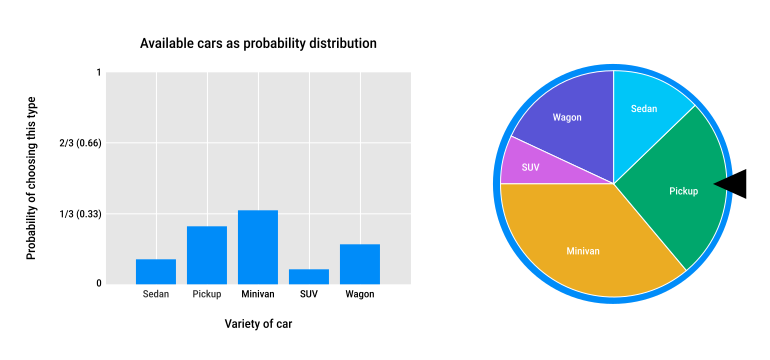
If we assign a category to 950 cars (sedan, pickup, minivan, SUV, wagon):

• the probability of each category is the number of objects in that category divided by the total
• these probabilities form a probability distribution, where all values range from 0 to 1 and sum to 1

A random variable is a function associated with a probability distribution:

• input: a probability distribution
• output:
  • a single value (e.g., sedan, pickup, minivan, SUV, or wagon)
  • the output is random but follows the probabilities given by the distribution

Selecting a value from a distribution is called drawing a value from the random variable.

Probability distributions are classified into two main categories:

1. continuous probability distribution
   • used when the outcomes can take any real value in a range (e.g., the amount of oil in a car)
   • also called a probability density function (pdf)
2. discrete probability distribution
   • used when the outcomes are countable and can only take a fixed number of possible values (e.g., vehicle types)
   • also called a probability mass function (pmf)

In practice, random values are generated by selecting a probability distribution and drawing a random variable from it.

Continuous distributions

The uniform distribution

Every value within a specific range is equally likely to be selected.

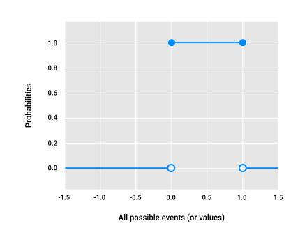
The most basic version is the uniform distribution from 0 to 1 (by convention here, a closed circle = the point is included):

Two key features:

1. fixed range:
   • we get 0 everywhere except between values 0 and 1
   • the distribution is called finite because it has a specific minimum and maximum
2. uniform likelihood:
   • every value in the range 0 to 1 is equally probable
   • this is why the graph is described as uniform, flat, or constant in the range 0 to 1

The normal distribution

Also called the Gaussian distribution or bell curve.

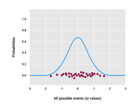
• when drawing random values from a normal distribution:
  • they cluster near the center, meaning those values have high probability
  • they are sparser where the curve is low, meaning those values have low probability
• the values approach 0 as we move away from the center, but never quite reach it:
  • we say the width of this distribution is infinite
  • in practice, values very close to 0 are treated as zero, effectively making the distribution finite

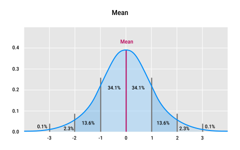
A normal distribution is defined by two numbers: the mean and the standard deviation.

Term	Explanation	Image
Mean (average)	Determines the center location of the peak. It's also the median and the mode (a special property of the normal distribution).
Standard deviation σ (écart type)	σ (lowercase sigma) is a unit of distance (like a step size) that measures how spread out the data are around the mean. To find it: start at the center of the peak move outward symmetrically until you enclose about 68 % of the area under the curve the distance from the center to either end of this interval is one standard deviation From −σ to +σ = two steps total distance, but still called within 1 standard deviation because we're only going −1σ away from the center in each direction. Extending further: by another standard deviation encloses 95 % of the area under the curve by another standard deviation encloses 99.7 % of the area under the curve this is known as the three-sigma-rule or 68-95-99.7 rule For 1,000 samples drawn from a normal distribution: about 680 are within ±1σ (one standard deviation) about 950 are within ±2σ (two standard deviations) about 997 are within ±3σ (three standard deviations)

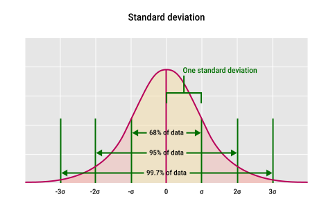
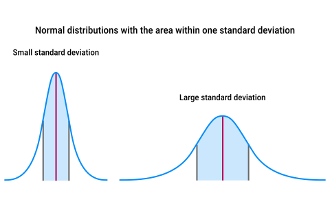
Sometimes, instead of standard deviation, the variance is used for convenience:

• variance is the square of the standard deviation (σ²)
• the general interpretation is the same: larger variances indicate more spread-out curves

The normal distribution appears frequently because it naturally describes many real-world observations.

Discrete distributions

The Bernoulli distribution

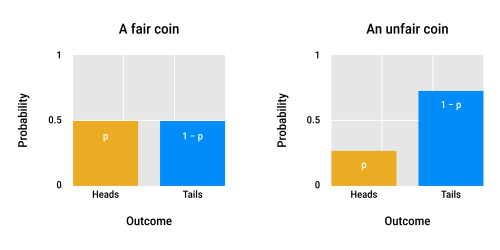
Simple discrete distribution that produces only two possible outcomes: 0 and 1.

A common example is a coin flip:

• 1 might represent heads with probability p
• 0 represents tails with probability 1 − p

The Multinoulli distribution (or categorical distribution)

Extends the Bernoulli distribution for more than two outcomes, where an event will have one of K possible outcomes (e.g., a 20-sided die).

This kind of distribution is important for training classifiers that sort inputs into many classes.

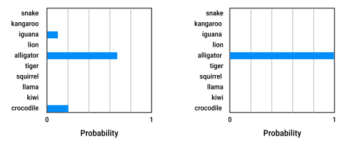
The output is a list where all entries are 0 except for the chosen category, which is 1.

For example:

• we have a photo of an alligator
• our algorithm is not sure what the image is and guesses several possible animals (left image)
• but what we really want is just one answer: the alligator (right image)

Expectation, dependence, and independence

Expected value

The average (or mean) of a list of numbers is called the expected value.

This is useful in many situations:

• suppose we want a random number between -1 and 1
• if the expected value is 0
• then the set of values is balanced: they're equally likely to be positive or negative

Dependence

Independent variables don't depend on each other.

Dependent variables do depend on each other:

• imagine we have different fur length distributions for animals like dogs, cats, and hamsters
• first, we randomly pick an animal
  • this choice is independent: it doesn't rely on anything else
• then, based on the animal, we choose a fur length from the right distribution
  • this choice is dependent: the fur length depends on which animal we picked

Independent and identically distributed variables

Values called i.i.d. (independent and identically distributed) are:

• values drawn repeatedly from the same distribution
• with no relationship between the values (they're independent)

Sampling and replacement

It's useful to build new datasets from existing ones by randomly selecting some of the elements of the existing set.

Selection with replacement (SWR)

We make a copy of each item we select, so the original stays in the dataset:

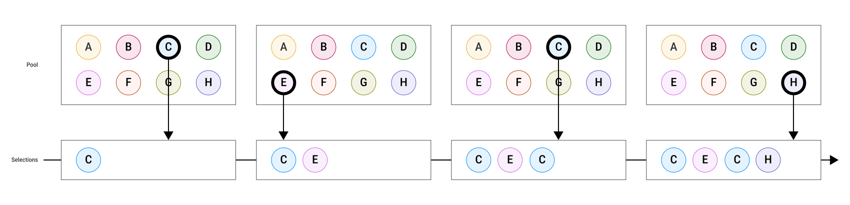
• we might pick the same item more than once
  • in the worst case, all picks could be the same item
• the original dataset stays the same, so the new dataset can be:
  • smaller than the original
  • the same size
  • bigger
• statistically:
  • each selection is independent
  • there is no history:
    • what you pick before doesn't change the chances next time
    • every item has the same chance every time

This is called selection with replacement because we can think of it as:

1. removing the object
2. making a copy
3. replacing the original

Selection without replacement (SWOR)

We remove the item we pick from the original dataset:

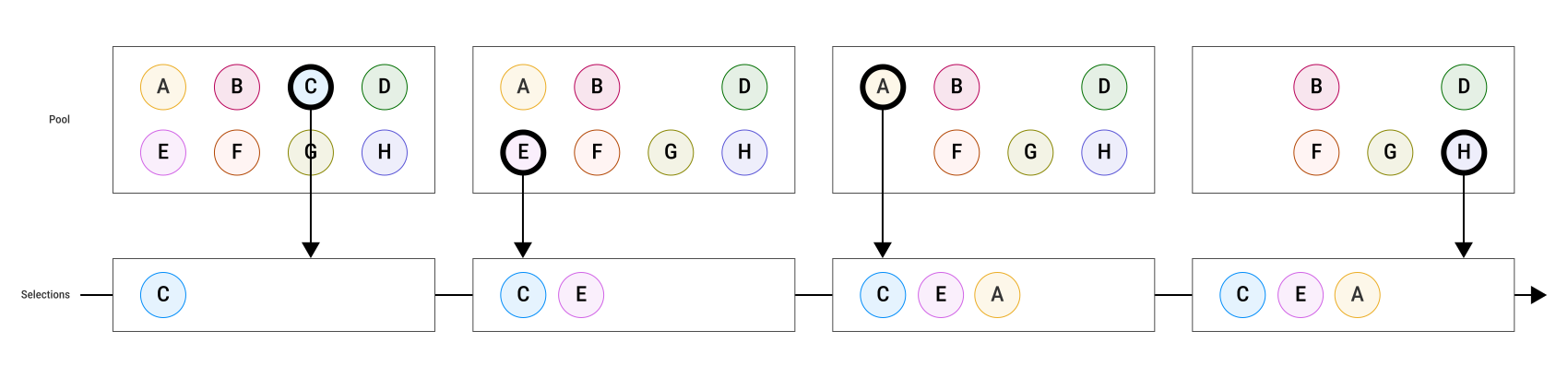
• you can't pick the same item more than once
• the original dataset gets smaller, so the new dataset can be:
  • smaller than the original
  • the same size
  • but never bigger
• statistically:
  • each selection is dependent on the ones before
  • there is history:
    • our selections are affected by previous choices
    • when we remove an element, the odds of selecting a remaining element go up
      • start with 8 items → each has a 1 in 8 chance of being picked
      • pick 1 → now 7 items → each has a 1 in 7 chance of being picked
      • and so on…

Bootstrapping

Bootstrapping (or bagging, or resampling) is a statistical technique used to estimate properties of a large population by working with smaller, manageable samples.

Bootstrapping involves two steps:

1. create a sample set from the population using sampling without replacement (SWOR)
2. resample that sample set many times with replacement (SWR) to create multiple new samples called bootstraps

Example: estimating the average height of babies

• imagine a "large" population of 5,000 baby lengths, ranging from 0 to 1,000 mm:
  • suppose the true mean is about 500 mm (50 cm)
  • in reality, this value is unknown, since computing statistics for large populations is often impractical
• SWOR: randomly select 500 measurements from the population to create a representative sample set
  • compute its mean to estimate the mean of the entire population
  • sample mean ≈ 490 mm
  • but how accurate is this estimate?
• SWR: create 1,000 bootstraps from this sample, each with 20 elements
  • compute the mean for each bootstrap sample

Histogram of the 1,000 bootstrap means:

• X-axis → mean values (from 0–1000 mm)
• Y-axis → how many bootstraps produced that mean

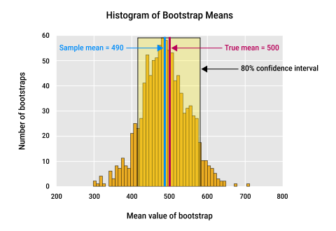
• bootstrapping helps estimate the accuracy of the sample mean (490 mm):
  • each bootstrap gives a mean, producing a distribution of possible means
  • this distribution is typically bell-shaped and centered near the true population mean because most bootstrap means are close to the true mean
  • the spread of this distribution reflects how much the estimate can vary
• to find the values we're 80% confident brackets the mean of the population:
  • remove the lowest 10% and highest 10% of bootstrap means
  • the remaining middle 80% forms the confidence interval ≈ 410–560 mm
  • we are 80% confident that the mean of the population is between 410 and 560 mm
  • this interval quantifies the uncertainty in our estimate

Bootstrapping is useful:

• even with populations of millions of measurements, we can use small bootstraps (like 10 or 20 items each)
• small bootstraps are fast to process
• creating many bootstraps (thousands) improves the precision of confidence intervals

Covariance and correlation

Variables can have relationships with each other:

• negative relationship: as one increases, the other decreases (e.g., higher temperature → lower chance of snow)
• positive relationship: as one increases, the other also increases (e.g., higher temperature → more people swimming)

Identifying and measuring these relationships is useful:

• strongly related variables may be redundant
• removing redundancy can speed up training and improve results

To measure these relationships, we use covariance and correlation.

Covariance

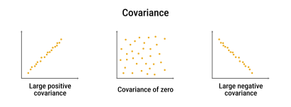
Two variables covary when one variable's value increases or decreases and the other does the same by a fixed multiple of that amount.

A number called the covariance measures:

• the strength of their connection
• or the consistency with which they vary together (covary)

The sign of the covariance tells us the direction of the relationship:

• positive → variables increase together
• negative → one increases as the other decreases
• zero → no relationship

Correlation

Because of the way covariance is defined mathematically, it doesn't take into account relationships between the units of the two variables.

The correlation coefficient (or correlation) solves this problem to let us make these comparisons:

• it starts with the covariance
• but adds one extra step to make it unit-free
• the result is a number that does not depend on the units that were chosen for the variables
• it always falls between –1 and +1:
  • +1 → perfect positive correlation
  • -1 → perfect negative correlation
  • values near 0 → weak or no correlation

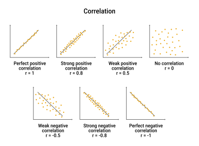
When two variables have a perfect positive or negative correlation (+1 or -1), the variables are linearly correlated.

Correlation is more useful because it isn't affected by the scale of the numbers.

Statistics don't tell us everything

The Anscombe's quartet is a famous example of how statistics can be misleading:

• there are four different sets of 2D points
• they all have the same mean, variance, correlation, and straight-line fit
• if we only looked at the statistics, we might think these four datasets were identical, but they're not

We shouldn't assume that statistics tell us everything about any data set.

Whenever we work with new data, it's important to:

• take the time to get to know the data
• compute statistics to summarize it
• draw plots and visualizations to see patterns and anomalies

High-dimensional spaces

A single sample (or piece of data) often contains many numbers called features. For example, a piece of fruit might be described by its weight, color, and size.

Each sample can be thought of as a point in a space, where each feature corresponds to one dimension:

• 1 feature → 1D (line)
• 2 features → 2D (plane)
• 3 features → 3D (cube)

Many datasets have far more features. For instance, a 1,000 x 1,000 grayscale image has 1,000,000 pixel values → a million dimensions.

We cannot visualize or imagine such high-dimensional spaces, but the mathematics and algorithms can handle such high-dimensional spaces.

While intuition from lower dimensions helps, high-dimensional spaces can behave in unexpected ways.