Overfitting and underfitting
Learning from limited examples involves balancing generalization and specificity:
- if a model is too general, it underfits: it doesn't learn from the training data well enough and performs poorly on new data
- if a model is too specific, it overfits: it excels on training data, but does poorly when presented with new data
Overfitting is the more common issue and is managed using regularization techniques.
Detecting and addressing overfitting
Overfitting happens when a model learns the training data too well (including its noise and specific details) so it struggles to make accurate predictions on new data.
Overfitting can be detected by monitoring the training error and the validation error (an estimate of how well the model is likely to perform on new data):
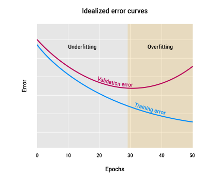
- underfitting → the model is too simple and misses important patterns
- overfitting → the model is too closely tailored to the training data
- it occurs when training error keeps decreasing but validation error stops improving or increases
- the model is learning training-specific details instead of learning general patterns
Example:
- a store owner uses a service that plays background music
- she adjusts the tempo throughout the day but finds it distracting to do so manually
- we're hired to build a system that adjusts the tempo automatically based on her preferences
- we collect data:
- each time she adjusts the tempo, we note the time and new tempo setting
- this is all the data we're going to get, no more
- we try to fit curves to this data
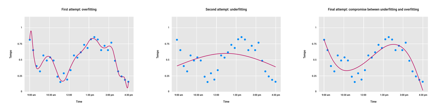
- first attempt — overfitting
- the curve is complex but matches her exact choices
- we program the system to follow this pattern but the tempo is changing too often and too dramatically
- the model has learned too many details about that one day's songs
- second attempt — underfitting
- we simplify the curve
- now it ignores important trends (like different preferences in the morning and afternoon)
- the model is too simple, the curve is underfitting the data
- final attempt — just right (compromise between underfitting and overfitting)
- a smoother curve captures the overall trend without copying every small detail
- this curve is not trying to match all of the data exactly but is getting a good feeling for the general trends
- the owner is happy
Good models strike a balance:
- not too simple → avoid underfitting
- not too complex → avoid overfitting
The main goal is to perform well on new data, not just the training data.
Early stopping (prevent overfitting)
When training a machine learning model:
- early in training, the model is underfitting
- it hasn't learned enough
- performance is poor on both training and validation data
- as training continues:
- both training and validation errors decrease
- eventually, the validation error starts to rise while training error keeps falling:
- this indicates overfitting
- the model is learning too much from the training data, including noise
Early stopping (or last-minute stopping):
- is a technique to prevent overfitting by halting training as soon as the validation error begins to increase, even if the training error could still be reduced further
- this captures the best model state (the point of optimal generalization) before overfitting occurs
In practice:
- error measurements are rarely smooth curves, they tend to be noisy and may temporarily move in the "wrong" direction
- this noise makes it difficult to find the exact right point to stop training
Regularization
While early stopping halts training once validation error starts rising, regularization aims to delay that rise so we can train longer and improve both training and validation performance.
Regularization is achieved by:
- forcing the values of the parameters used by the classifier to be in similar ranges to prevent any single parameter from dominating the model's decisions
- this encourages the model to rely on multiple features rather than a few idiosyncratic ones, improving generalization
- as a result, the model's decision boundaries become smoother and less complex
Implementation:
- the amount of regularization is controlled by a hyperparameter (lambda
λ)- higher
λ→ stronger regularization → smoother boundaries and simpler models - lower
λ→ less regularization → boundaries fit more precisely to the training data
- higher
- the optimal
λvaries by dataset and model, so it must be tuned experimentally
For multi-layer architectures, specialized regularization methods like dropout, batchnorm, layer norm, and weight regularization provide additional ways to control overfitting.
Bias and variance
Imagine we've been measuring daily wind speed on a mountain over several months.
The observed data shows:
- a lot of noise (day-to-day fluctuations)
- but also a clear underlying pattern that we assume can be described by a smooth "ideal" curve
Since the exact amount of noise is unknown, the goal is to approximate the underlying curve by trying to fit a curve that captures the general trend:
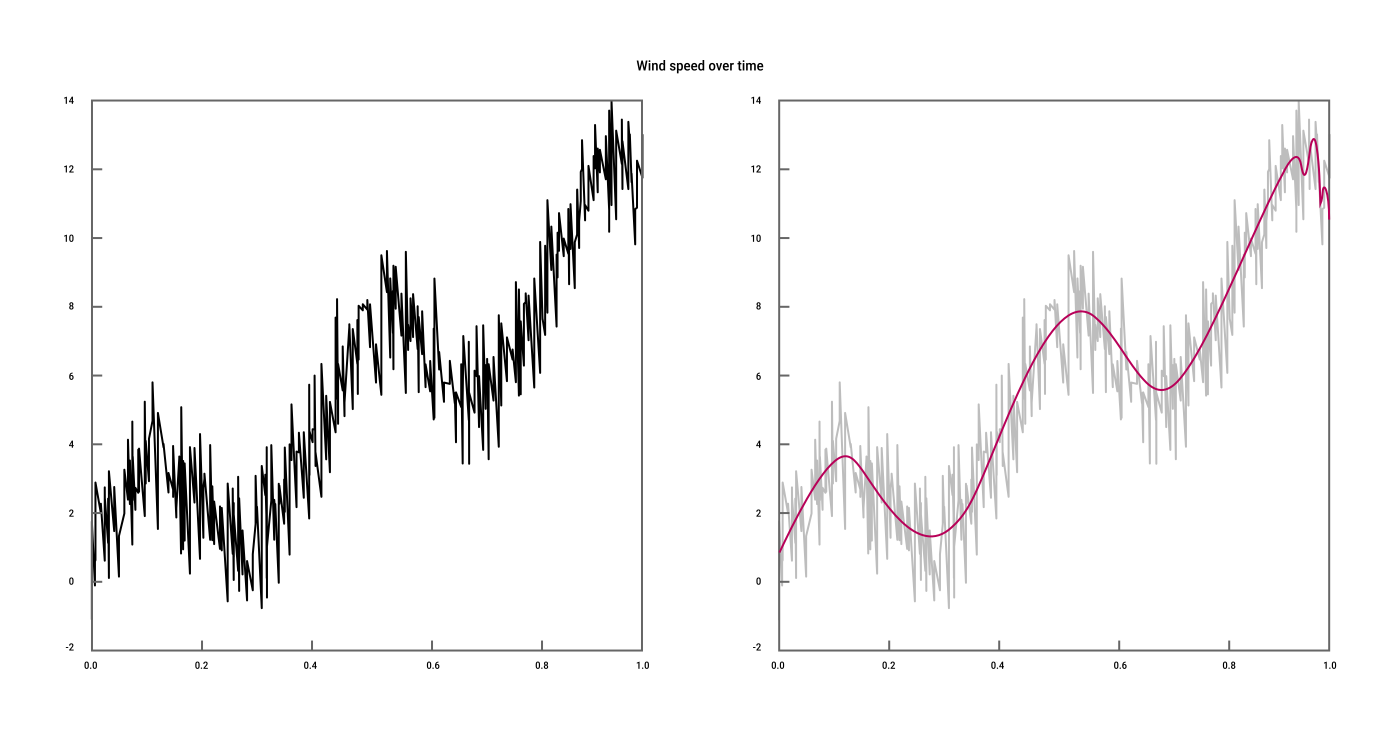
Bias and variance can explain why different curve-fitting choices succeed or fail at recovering the "ideal" underlying curve.
We generate smaller datasets by randomly sampling 30 points each and then fit simple and complex curves to them:
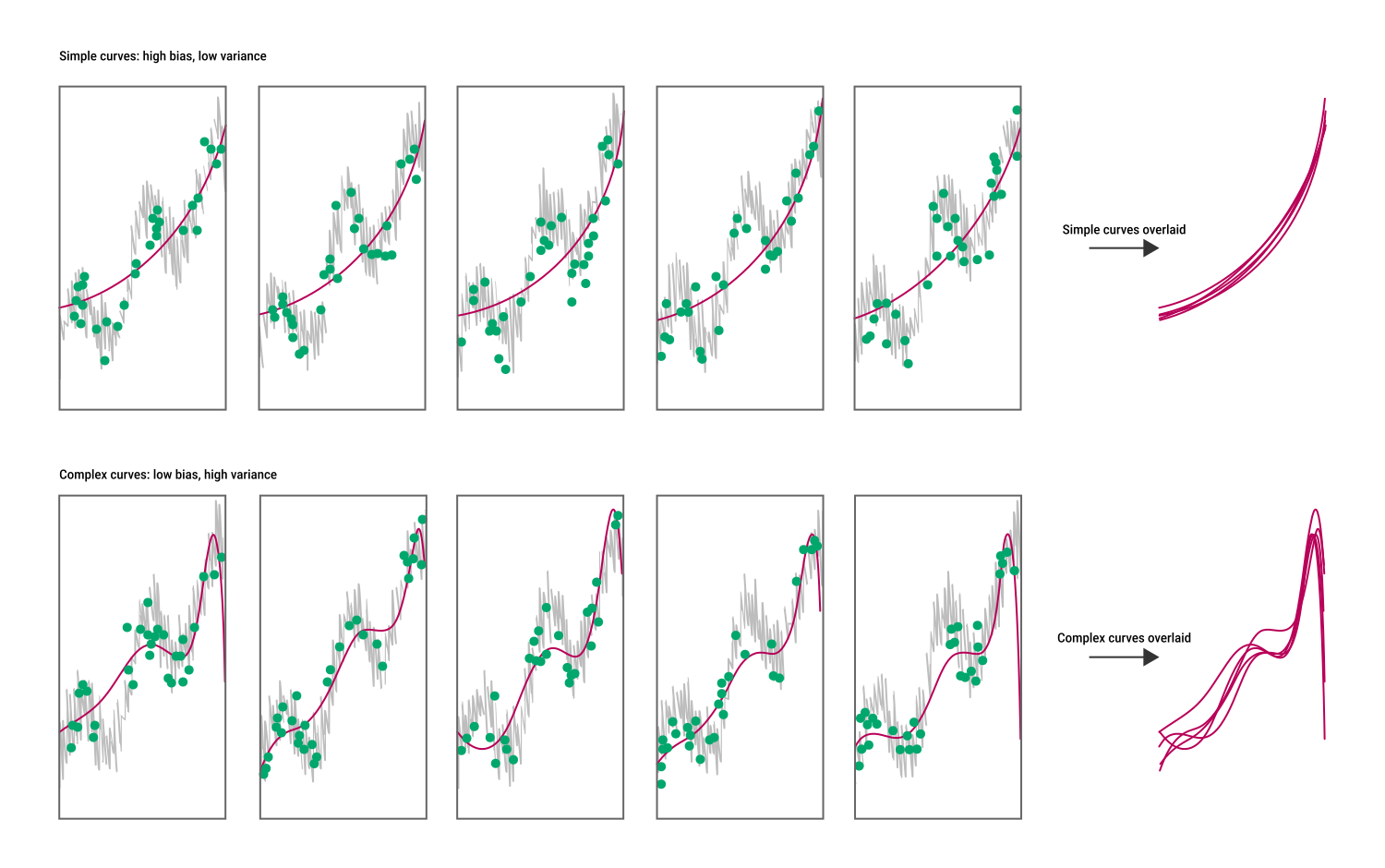
Simple curves have:
- a high bias:
- all curves look similar
- the model is too simple, so it can't capture all the important patterns (underfit)
- a low variance:
- the variance refers to how much the curves vary or differ
- when overlaid, the curves don't change much
- the individual curves aren't being influenced much by the data
Complex curves follow the data much more closely and have:
- a low bias:
- the curves have different shapes
- they are more influenced by the data
- a high variance:
- when overlaid, the curves vary a lot
- each curve is strongly influenced by its data, creating "high variance" (large differences) between curves
Bias and variance:
- bias and variance describe groups of curves, not single ones
- it doesn't make sense to discuss the bias and variance of just one curve
Bias and variance help explain underfitting and overfitting:
- early in training:
- models underfit (high bias, low variance)
- occurs with models that are too simple
- late in training:
- models may overfit (low bias, high variance)
- happens with models that follow training data too closely
Ideally, we'd like curves with a low bias and low variance, but in practice, when one goes down, the other often goes up.
The goal is to find the best bias-variance tradeoff for each specific situation.
In some applications:
- high variance is acceptable:
- if the training set is known to be fully representative of all future data
- so fitting it closely (low bias) is desirable
- high bias is acceptable:
- if the training data is not representative of future data
- so exact fitting doesn't matter
- stable, general behavior (low variance) is more important for future unseen data
Fitting a line with Bayes' rule
Bias and variance are concepts commonly used in frequentist analysis.
The Bayesian approach treats all possible curves as having probabilities, updating those probabilities as more data is collected, but never settling on a single "final true" answer.
We'll use Bayes' Rule to approximate the noisy atmospheric dataset with a straight line for simplicity.
Some tricks to make lines easier to visualize:
| Title | Explanation | Image |
|---|---|---|
|
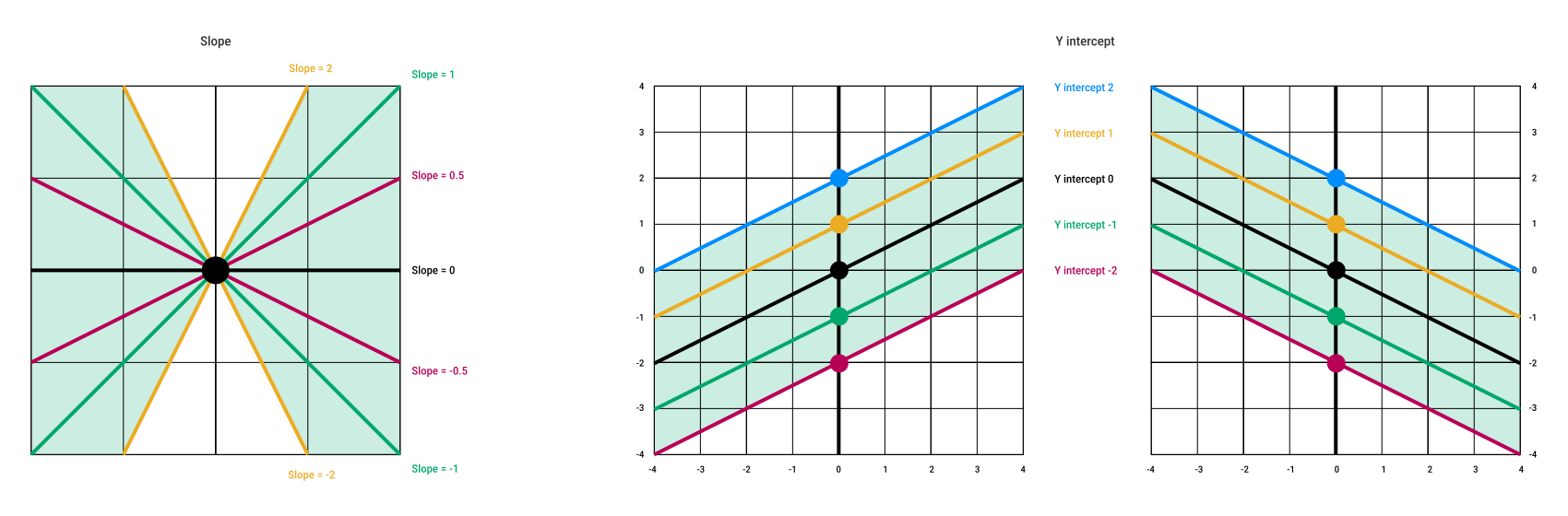
Slope–intercept form |
A line can be represented as a single point using two numbers:
|
|
|
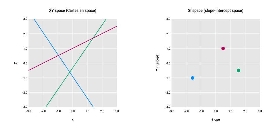
Dual representation |
XY and SI spaces enable a dual mapping between them:
This allows us to visualize many possible lines compactly. |
|
|
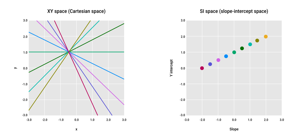
Elegant point about the dual representation |
If points are arranged along a line in SI space, the equation linking slope and intercept ensures that all the corresponding XY lines intersect at the same point. |
|
Bayesian curve fitting assigns a probability to every possible line based on how well it fits the data.
Example: likelihood of all possible straight lines for a single data point of the noisy dataset:
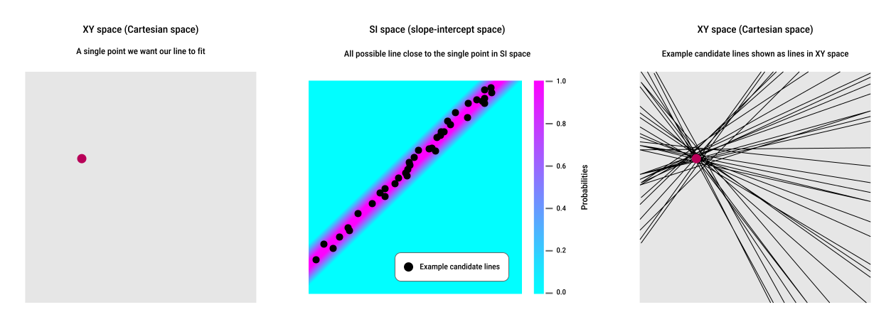
Full example: find the likelihood of all possible straight lines for the full noisy data set:
| Step | Image | Explanation |
|---|---|---|
| 1 | 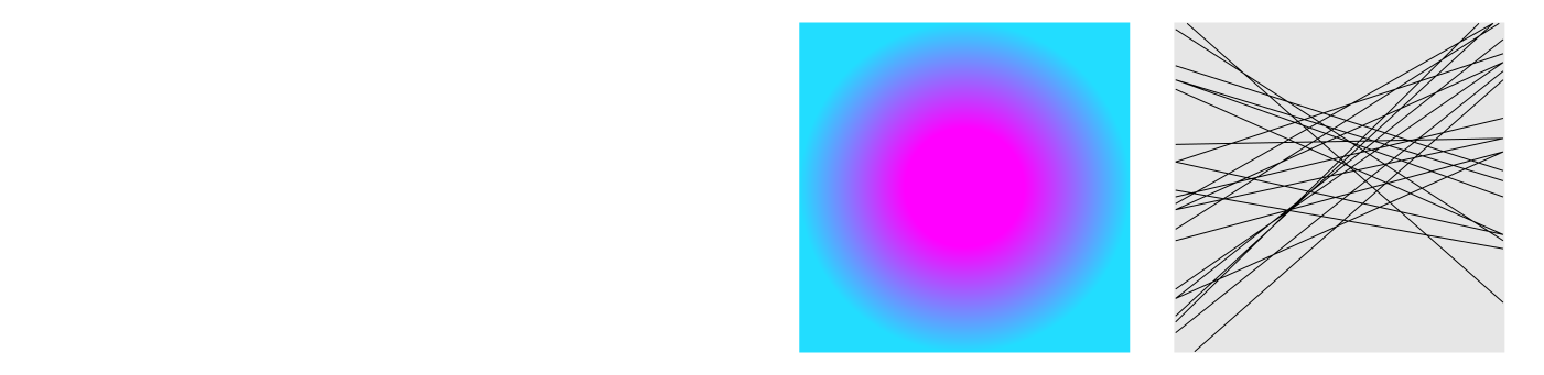 |
Left:
Right:
|
| 2 | 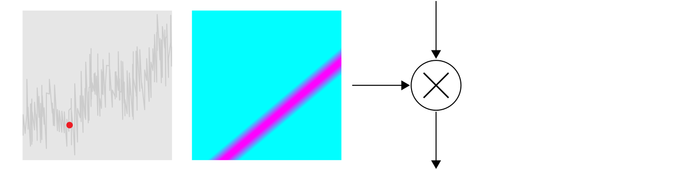 |
Left:
Right:
Apply Bayes' Rule: |
| 3 | 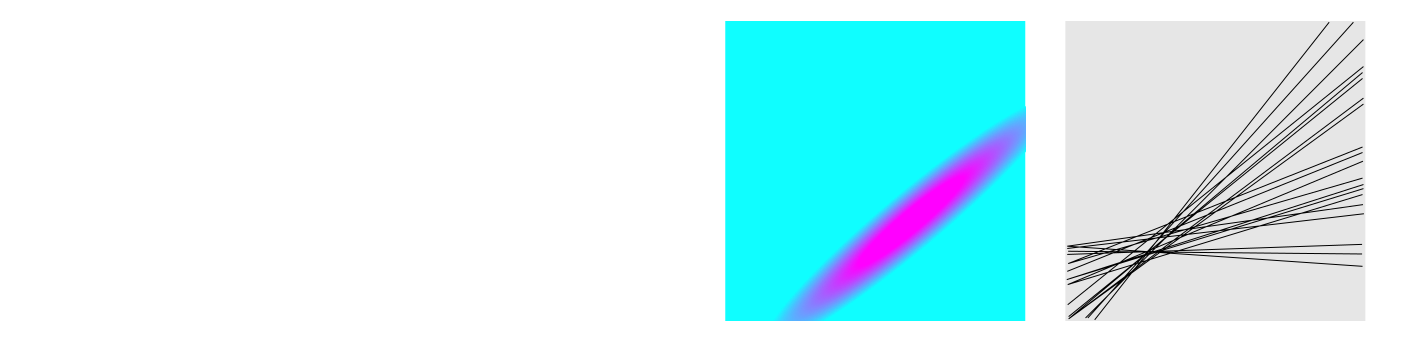 |
Left:
Right:
The posterior becomes the new prior. |
| 4 | 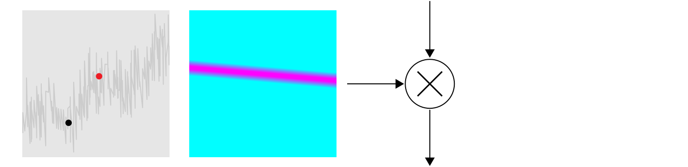 |
Left:
Right:
Apply Bayes' Rule: |
| 5 | 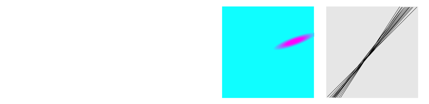 |
Left:
Right:
|
| 6 | 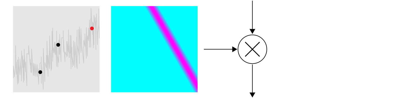 |
Repeat this process again and again. Each step refines the posterior further. Over time, the system converges toward a small set of lines that fit the data well. |
| 7 | 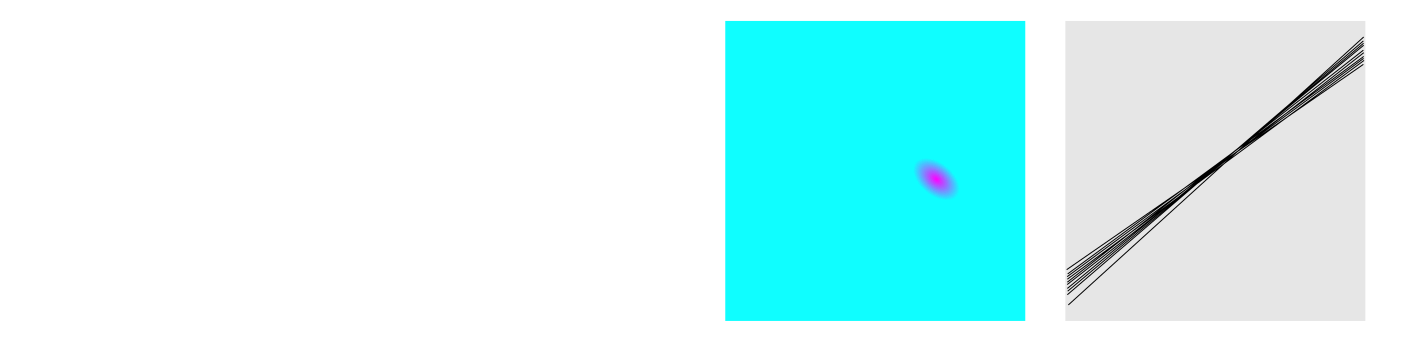 |
Bayes' Rule is useful in training a learning system:
- it allows a model to learn incrementally and update its beliefs based on new data
- as more data points are seen, the model's predictions become more precise
In Bayesian terms:
- every possible line has some probability
- the goal isn't to find a single "true" line but to describe how certain we are about each possible line
 Joint
Joint