Data preparation

Machine learning algorithms can only work as well as the data they're trained on.

Real-world data often contains errors, noise, or missing information. It must be cleaned before use.

Data preparation, or data cleaning, ensures that data is accurate, consistent, and suitable for learning algorithms.

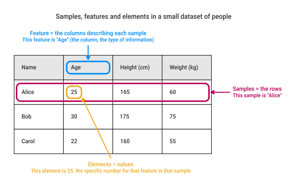
Dataset, samples, features and elements

A dataset is:

• a collection of samples
• each sample is described by features
• the elements are the actual numerical values of those features within each sample

Basic data cleaning

Simple ways to clean the data:

• fix text problems: correct typos, misspellings, and unprintable characters (in text data)
• remove duplicates
• ensure correct data formats:
  • e.g., scientific notation has no official format: 7e-3 vs. 7E-3
  • a program might misread 7e-3 as (7 x e) - 3 where e is Euler's constant
• look for missing data: try to patch the holes
• look for unusual data:
  • typos like a forgotten decimal point
  • or when someone forgot to delete an entry from a spreadsheet

These steps might seem basic, but they take time, and they're essential because clean, accurate data is the foundation for high-quality results.

The importance of consistency

Consistency is key.

Always apply the same data transformations to every dataset: training, validation, and real-world input.

If new data is handled differently, the model may focus on irrelevant features and make errors.

Types of data

Data can be one of two types:

1. numerical (quantitative) data
   • values are numbers (floating-point or integer)
   • they can be sorted
2. categorical data
   • values are not numbers (often strings)
   • two subtypes:
     1. ordinal data: has a clear order, so it can be sorted
        • e.g., rainbow colors (red → orange → … → violet) have a natural order
     2. nominal data: has no natural order
        • e.g., a list of desktop items (paper clip, stapler, pencil sharpener, etc.)
        • nominal data can be converted to ordinal by defining a custom order

Since machine learning models require numeric inputs, all categorical data must be converted to numbers before training.

One-hot encoding

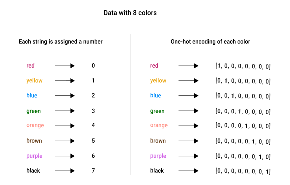
Data is often labeled with a single integer (e.g., class toaster = 3), but classifiers output a list of confidence values.

One-hot encoding converts a class label (like 3) into a list of numbers so it can be compared directly with a classifier's output:

• the list length equals the number of classes
• all values are 0 except for a single 1 at the index corresponding to the class

Example:

Normalizing and standardizing

Features often have very different numerical ranges.

Example of range of data on a herd of African bush elephants:

1. age in hours: 0 - 420,000
2. weight in tons: 0 - 7
3. tail length in centimeters: 120 - 155
4. age relative to the historical mean age (hours): -210,000 - 210,000

These ranges are very different and can affect how machine learning algorithms process the data:

• larger numbers can have more influence on the model than smaller ones
• some values can be negative, which adds complexity

To make algorithms work better, we want all features to be roughly comparable in scale.

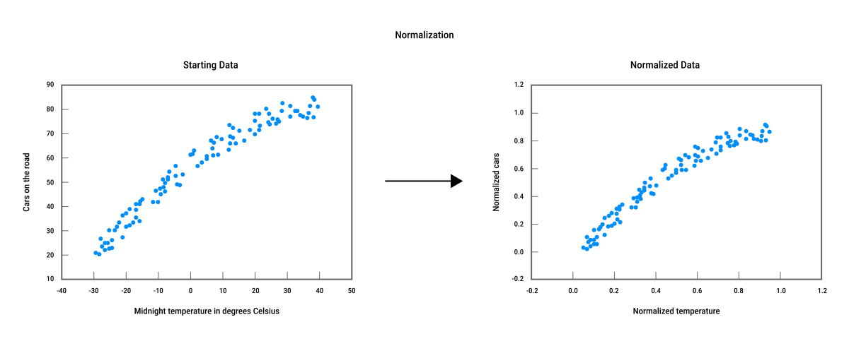
Normalization

Normalization scales data features into a specific range, usually [-1,1] or [0,1].

This ensures all features contribute equally to the learning process.

Standardization

Standardization is a two-step feature-scaling process:

1. mean normalization: each feature is shifted so its mean becomes 0 (centered at the origin)
2. variance normalization: each feature is scaled so its standard deviation becomes 1, meaning about 68% of the values fall between -1 and 1

Unlike simple normalization, standardization doesn't limit values to a specific range, some may go outside the range [-1, 1].

The process can distort the shape of the data, especially if the original distribution isn't normally distributed.

Types of transformations

Transformations can be:

• univariate:
  • work on one feature at a time, independently of others
  • often works better when features are independent
• multivariate:
  • handle multiple features together as a group
  • the most extreme (and most common) version is to transform all features simultaneously
  • often works better when features are related (like time-series temperature readings)

Slice processing

Slice processing refers to different ways of selecting ("slicing") and operating on parts of a dataset:

Method	Description	Example
Samplewise processing (slice by rows)	Each sample is scaled independently. Appropriate when all features are aspects of the same thing.	Audio data (features in each sample = amplitude of the audio at successive moments): 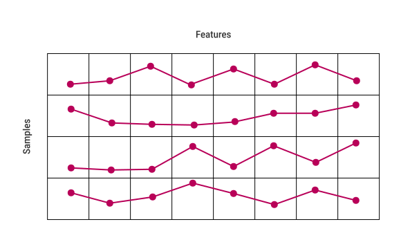all the features in a single sample are scaled to the range [0,1], normalizing its loudest value to 1 and quietest to 0
Featurewise processing (slice by columns)	Each feature is scaled independently. Appropriate when samples contain different types of measurements.	Weather measurements (temperature, rainfall, wind speed and humidity): 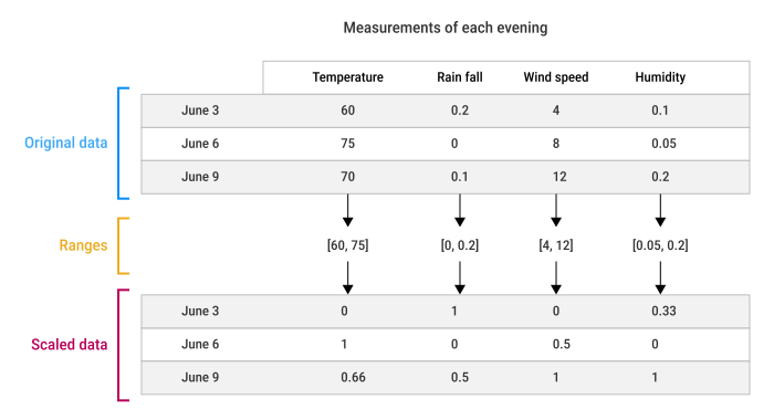scaling samplewise doesn't make sense because the units are incompatible
Elementwise processing (slice by values)	Each element is scaled independently. Appropriate when all data is of the same type and needs a consistent change.	Converting heights from inches to millimeters.

Inverse transformations

Sometimes we need to undo (invert) transformations so we can interpret results in the original data scale.

Example with predicting rush-hour traffic from temperature:

1. collect data over several months:
   • nightly temperatures at midnight
   • cars count on the highway the next morning (7–8 AM)
2. transformation (scaling):
   • the model scales both features into the range [0,1]
3. training:
   • train the model only on scaled data
4. using the model on unseen data:
   • input: -10° Celsius → scaled to 0.29
   • output: traffic density of 0.32
   • we must apply the inverse transformation to interpret the data: 0.32 → 39 cars

Handling out-of-range values:

• inputs beyond the training range (like -50°C) will produce values outside [0,1], which is acceptable since scaling is mainly used to improve training efficiency
• however, outputs must still be interpreted carefully, as unrealistic predictions (like negative numbers of cars) should not be used literally for decision-making

Information leakage in cross-validation

Information leakage happens when a model accidentally "sees" data it shouldn't during training.

A common source is data transformations in cross-validation:

• scaling or normalizing the entire dataset before splitting into folds lets the transformation "knows" the min and max values of the validation data
• this is information leakage, because the validation data influences the transformation by "leaking" into training data
• as a result, the model appears more accurate than it truly is

To prevent leakage:

• for each fold, remove the validation data
• compute the transformation using only the training data
• retain that transformation
• apply the transformation to both the training and validation data

Modern libraries handle this automatically.

Shrinking the dataset

Feature selection

Feature selection (or feature filtering) removes irrelevant, redundant, or unhelpful features from a dataset.

Example:

• we're hand-labeling images of elephants and recording features like size and species
• for some reason nobody can remember there's a field for "the number of heads" but all elephants have only one head
• this feature is useless and slows down processing, so it should be removed

Similarly, features that are highly correlated may be redundant. Removing one won't lose information.

Most libraries can estimate the effect of removing each field from the database.

Because removing a feature is a transformation, any feature removed from the training set must also be removed from all future data.

Dimensionality reduction

Dimensionality reduction reduces the number of features by combining related ones into fewer, more informative ones.

For example, the body mass index (BMI) is a single number that combines a person's height and weight that still reflects useful health information.

There are tools that can automatically learn how to combine features with minimal impact on model performance, such as Principal Component Analysis (PCA) and Autoencoders, which create compact representations of high-dimensional data.

Principal Component Analysis (PCA)

Principal component analysis (PCA) is a mathematical technique used to reduce the number of features (dimensions) in a dataset while keeping as much of the original information as possible.

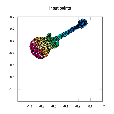
Using PCA to reduce 2D data (x and y) into 1D data that still represents both (think of this like BMI):

Step	Explanation	Image
Data	A two-dimensional guitar dataset: the guitar shape is arbitrarily chosen because it helps see what happens to the points colors are just for visualization and don't carry any special meaning the points are typically the results of x and y measurements (like tempo and volume)
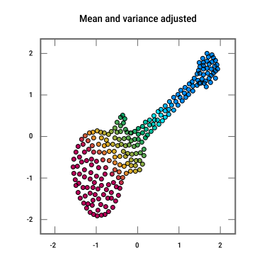
Normalization	Normalize the data so that each feature has a mean of 0 and a standard deviation of 1.
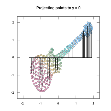
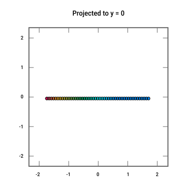
A bad projection example	Project the data straight onto the x-axis: the horizontal line is the projection line each point is projected directly onto this line (paths for about 25% of the points are shown)
	This 1D projection throws away all the y-information, like calculating BMI using only weight.
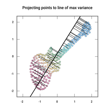
The correct PCA projection	PCA finds the best direction to project the data: the line is rotated until it's passing through the direction of maximum variance this is the line along which the data varies the most Each data point is then projected perpendicularly onto this new line (paths for about 25% of the points are shown).
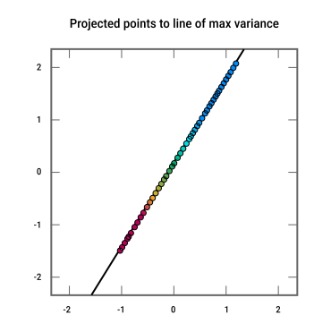
	This 1D projection captures information from both x and y and better represents the original dataset.
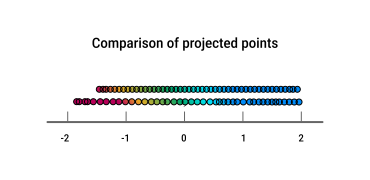
Result	The previous line is rotated to lie on the x-axis so it can be compared. The PCA is not just longer, but the points are also distributed differently.

All these steps are carried out automatically by machine learning libraries.

Reducing dimensions means some information is lost, so there's always a trade-off between simplicity and accuracy.

PCA can be applied to data with any number of dimensions, sometimes reducing the dimensionality of the data by tens or more.

Key questions when using PCA:

1. how many dimensions should we try to compress?
   • too few → training and evaluation are going to be inefficient
   • too many → you risk eliminating important information that should have been kept
2. which features should be combined, and how?

The hyperparameter k is used for the number of dimensions left after PCA:

• in the guitar example, k was 1
• to pick the best value for k:
  • try different values and compare results
  • or use automated hyperparameter search tools provided by libraries
• note: k is used for lots of different things in machine learning, so pay attention to the context

PCA for simple images

How it works:

Step	Explanation	Image
Data	Six grayscale bitmap images of 1,000 x 1,000 (= 1 million) pixels each. Problem: storing and working with that many numbers per image is expensive.
Shared component	Instead of storing millions of pixel values, PCA finds a small set of shared component images that capture the main patterns. In this example, 3 common parts are shared by all images.
Images as weighted combinations	Each original image can be created by: taking each common part scaling it by a number (here an opacity value) adding them together Example to obtain the first image: take 20 percent of the circle add 70 percent of the vertical box add 40 percent of the horizontal box
Weights	These scaling factors are the weights. Some weights may be negative.
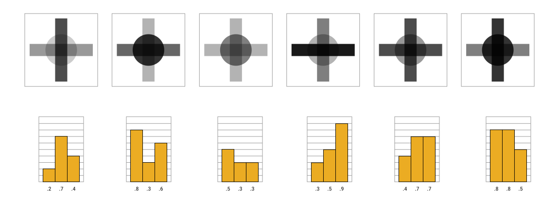
Result	We only store: three common parts or "principal components" the weights for each image (positive or negative) Here: 3 component images → ~3 MB 1,000 images × 3 weights/image = 3,000 values ≈ 0.001 megabytes → negligible

Images are usually standardized before applying PCA.

PCA for real images

Step	Explanation	Image
Data	Six real husky images: each 45x64 pixels (to make the processing easier to see) manually aligned so key facial features pixels (eyes, nose) represent similar parts of a dog
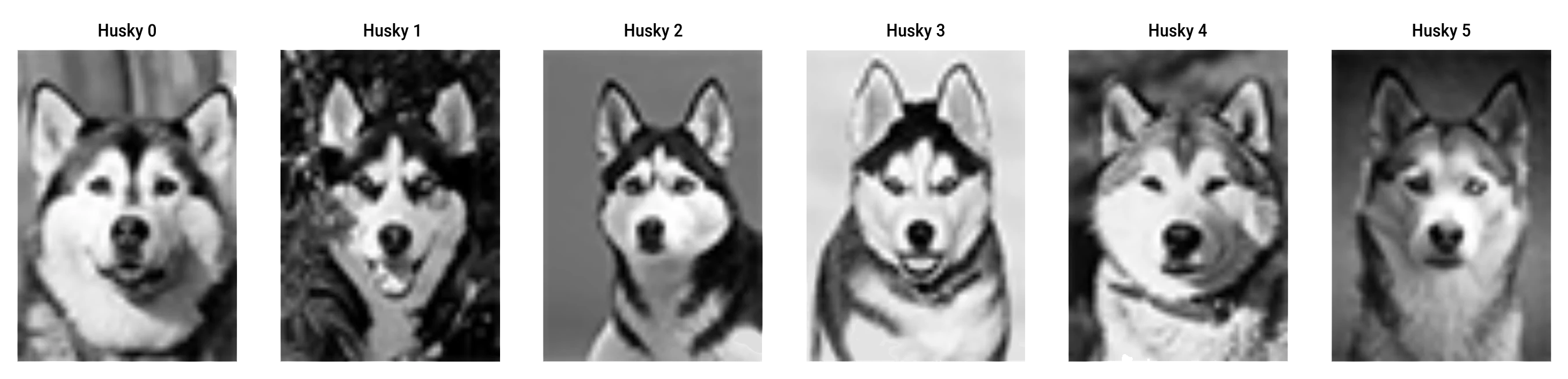
Data augmentation	6 images isn't enough for training. Data augmentation is used to expand the dataset to 4,000 dog images: each image is copied and randomly shifted, rotated and flipped horizontally.
Standardization	Each pixel across the 4,000 images is standardized to have zero mean and unit variance.
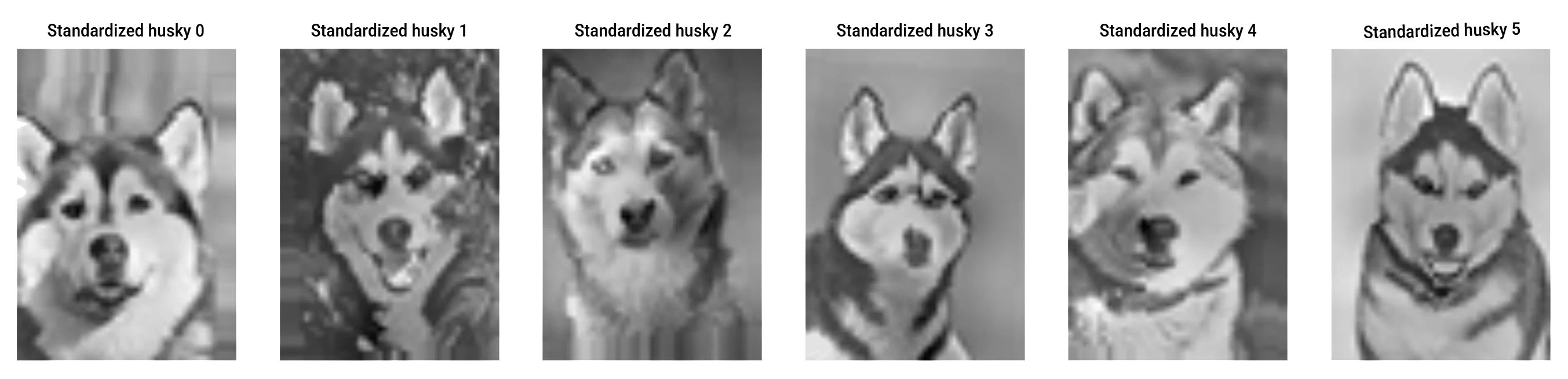
Train PCA	PCA is trained on the full augmented dataset. We start by arbitrarily asking it to find 12 eigenvectors (principal components) called "eigendogs" for fun. Each eigendog is a sort of "average" image that captures important variation patterns: 1st eigendog: captures broad, general features subsequent eigendogs: capture finer details
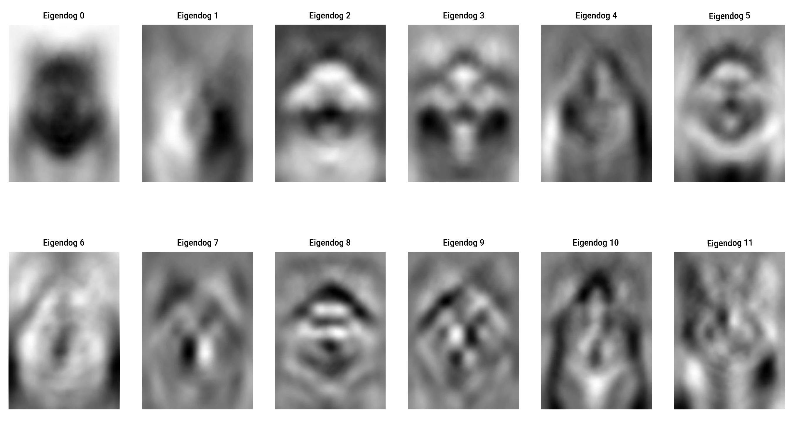
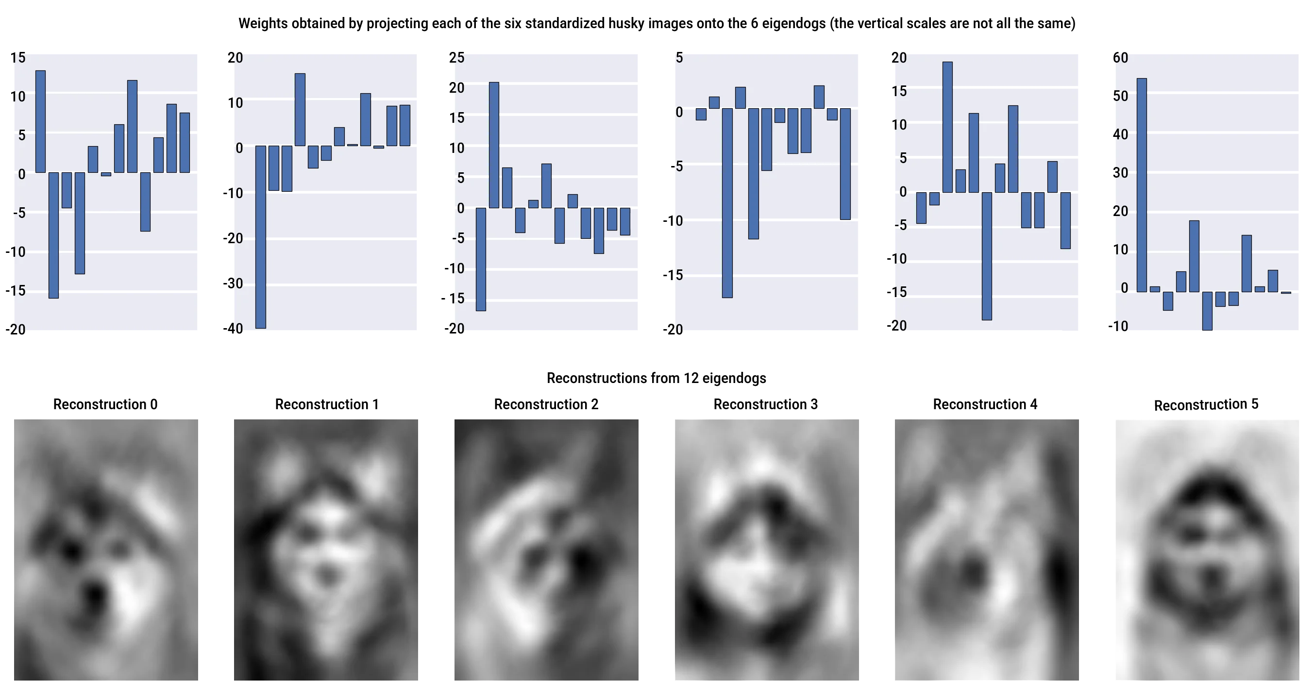
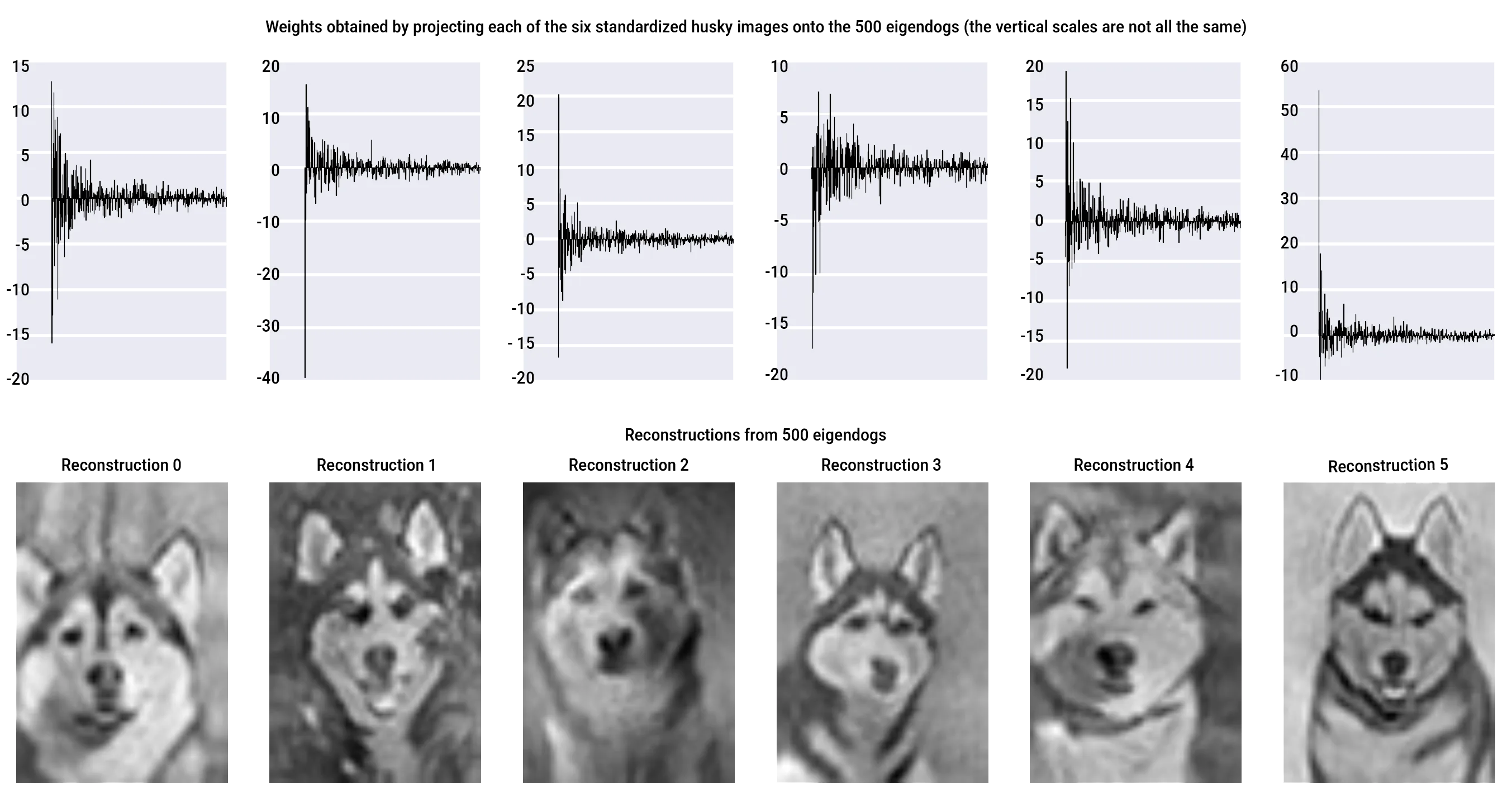
Reconstructing images	After eigendogs exist, each image (training or new) is standardized and projected onto each eigendog via a dot product, producing one weight per eigendog. These weights quantify how strongly each eigendog contributes to the image. Any image can be approximately reconstructed by forming a weighted sum of the eigendogs using these weights. For example, the six original husky images are reconstructed using different numbers of eigendogs: using 12 eigendogs: reconstructions are blurry but recognizable using 100 eigendogs: improved clarity using 500 eigendogs: reconstructions very close to the originals Increasing the number of eigendogs continuously improves reconstruction quality.
Result	Instead of storing all pixel data, we only need to store 100–500 PCA weights.

Although we used image reconstruction as a demonstration tool to show what PCA captures, PCA is not primarily used for reconstruction.

Its main benefit is dimensionality reduction:

• it compresses data into a much smaller set of meaningful values (PCA weights)
• this greatly reduces computational load while preserving essential features (faster algorithms)

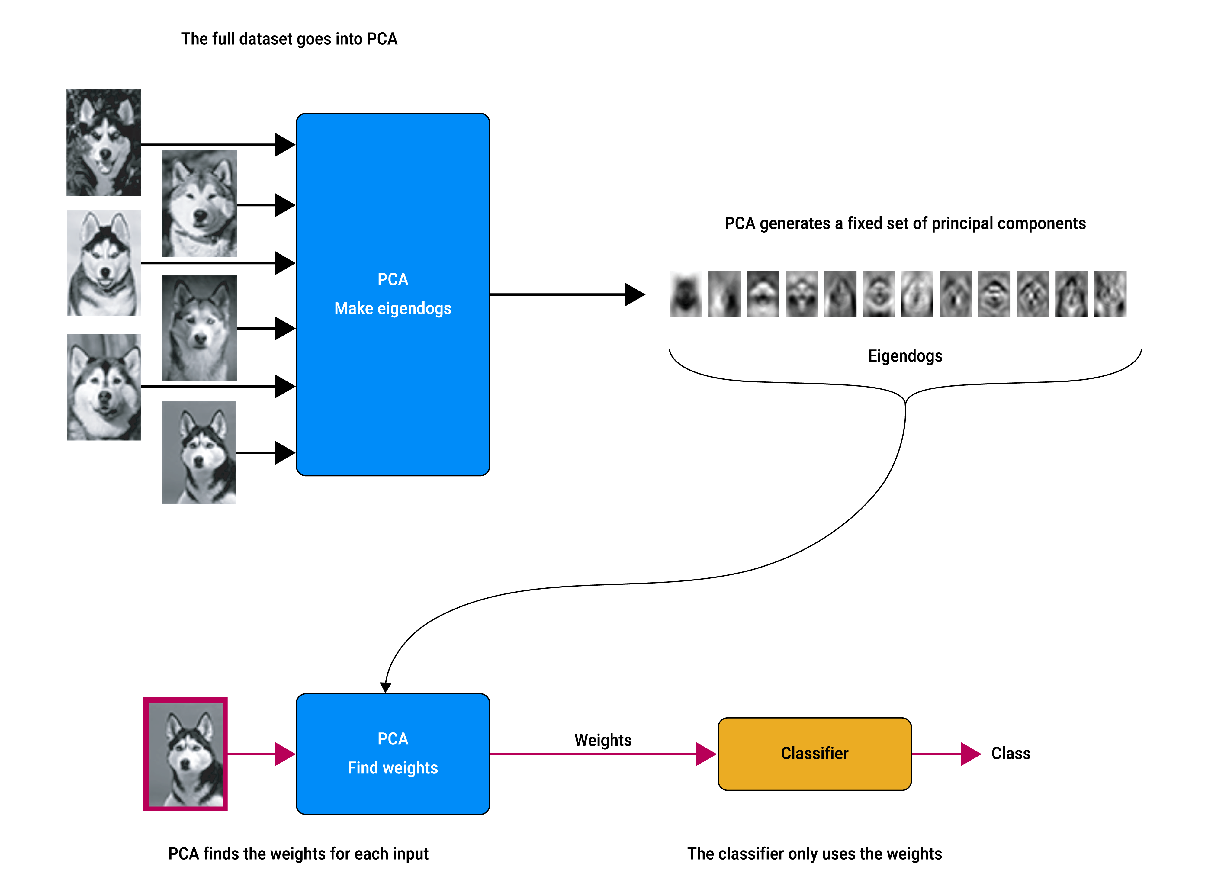
A classifier never sees the raw image or eigendogs but just the weight vector, which it uses to find the input's class: