Classifiers

There are 4 key classification algorithms.

For simplicity, examples use 2D data with two classes, but classifiers can handle high-dimensional data.

Types of classifiers

1. nonparametric classifiers
   • have no assumptions about the data's structure
   • learn directly from the data to find boundaries that separate different classes
   • like k-NN or decision trees
2. parametric classifiers
   • assume a specific data structure (e.g., a normal distribution)
   • then focus on finding the best parameters to fit that model
   • like SVM or naive bayes

This distinction is more conceptual than absolute but helps to classify algorithms.

k-nearest neighbors

k-Nearest Neighbors (kNN) is a nonparametric, supervised classification algorithm.

Core idea:

• all labeled training data is stored
• a new sample is classified using the most common class among its k closest neighbors

k is a hyperparameter chosen before training:

• it controls how many neighbors influence the classification
• choosing k is critical and requires experimentation

Classification is based purely on geometry:

• find the k nearest neighbors to the new sample
• count their classes
• assign the most common class

Example of different k values for a new sample (star) placed among labeled samples (circles, squares, triangles):

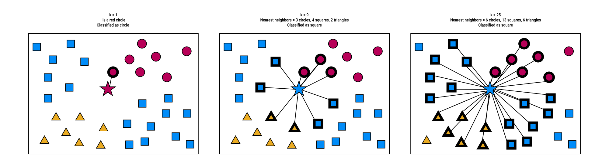
kNN is sensitive to data distribution, it works best when data points have many close neighbors.

kNN becomes less practical when:

• neighbors are far apart (sparse data)
• the dataset is high-dimensional (due to the "curse of dimensionality")

Decision trees

Introduction to trees

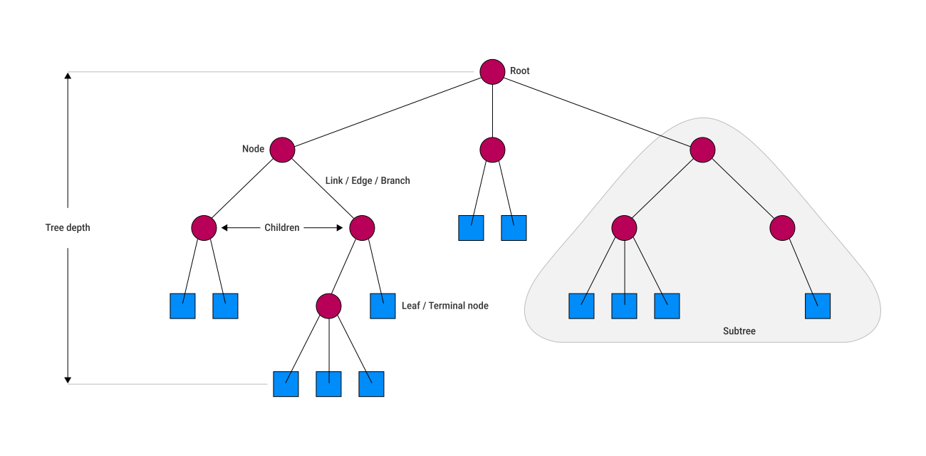
Term	Definition
Root	The topmost node.
Node	A decision point.
Link / Edge / Branch	A line connecting nodes.
Leaves / Terminal nodes	The bottom nodes that give the final answer.
Children	Nodes below a parent node are its children: immediate children: directly connected distant children: further down the tree
Depth	Every node has a depth: it's the smallest number of steps to reach the root root = depth 0
Siblings	Children with the same parent are siblings.
Subtree	A subtree includes a chosen node and all of its children.
Balanced / Unbalanced	If a tree has a perfectly symmetrical shape, it's balanced. Otherwise, it's unbalanced.

Using decision trees

Decision trees can be:

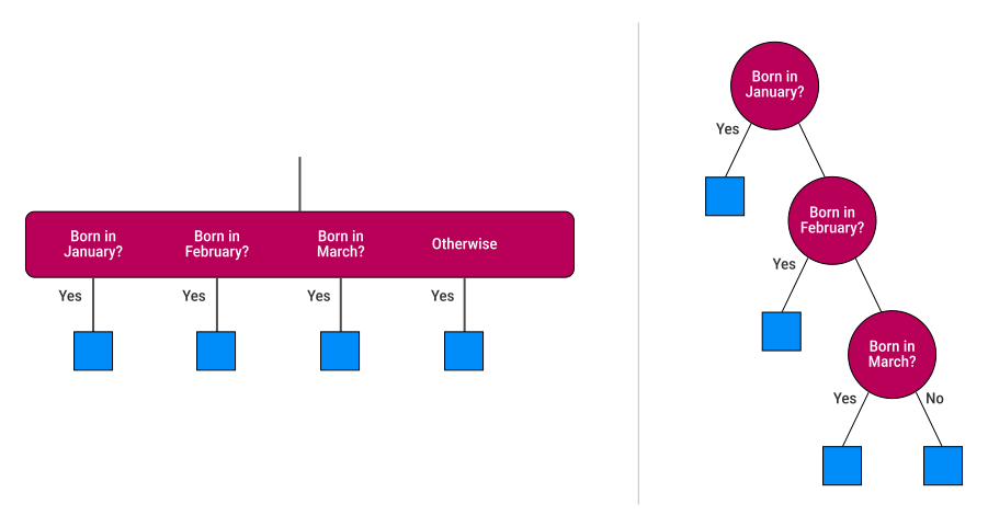
• binary: each node has two children (like yes/no)
• bushy: each node can have more than two children

Bushy trees can be converted into binary ones (simpler for algorithms to handle):

Using trees for classification:

• a decision tree classifies data at each node using tests based on features
• each decision splits the data into smaller groups until each leaf node contains samples from only one class
• the full method is called categorical variable decision trees

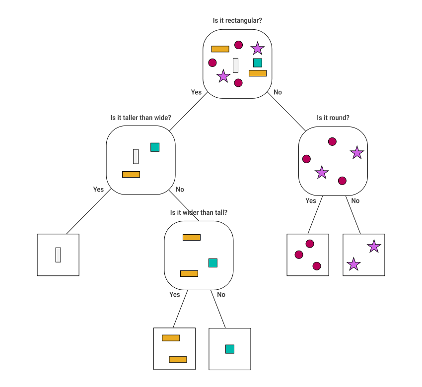
When groups aren't pure (i.e., mixed classes), the tree can output class probabilities instead of a single hard label.

Decision trees are popular because they are transparent and explainable: each classification can be traced through a sequence of human-understandable decisions.

However, transparency does not guarantee fairness, as the criteria used may still be biased.

Overfitting trees

The tree-building process is a learning algorithm that automatically constructs the tree from data.

When data is well-separated (like a "two-moons" dataset):

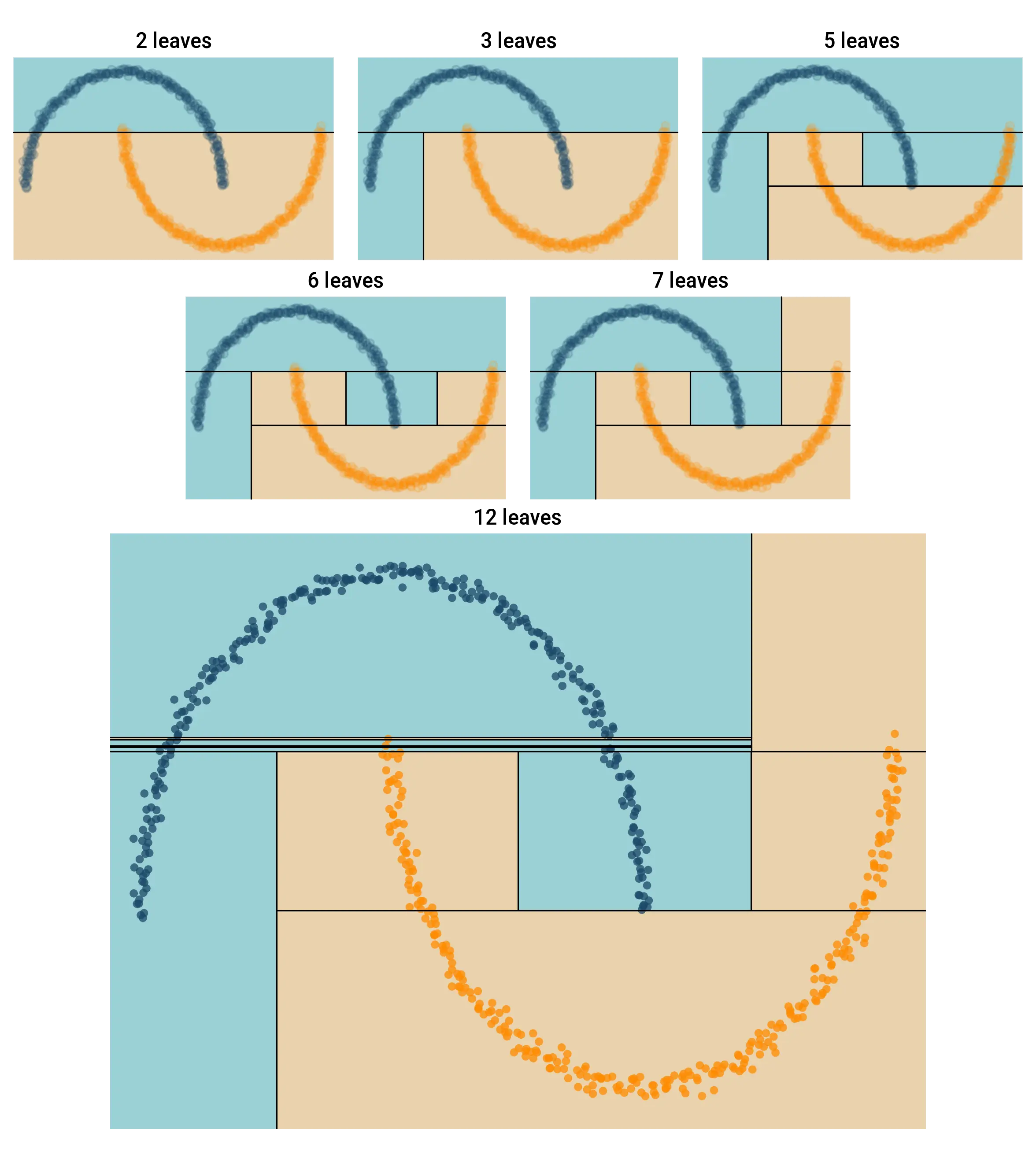
• the tree starts with large, simple regions and recursively refines them into smaller and more precise regions
• at the end, a small tree of 12 leaves can correctly classify all samples:
  • each node corresponds to a box
  • the entire region corresponds to the root
• but note the two horizontal thin rectangles when the tree has 12 boxes:
  • they capture a few orange points between blue ones
  • this indicates overfitting leading to misclassification of future samples in those regions

Decision trees are highly sensitive to the training data:

• each split depends on the exact training samples
• changing even a small number of training samples can alter where splits occur
• these altered splits can lead to a significantly different tree structure

This sensitivity leads to overfitting, especially with noisy data, where the boundary between classes is not clear:

• trees grow very deep and complex (e.g., 100 leaves) just to classify a few scattered points correctly
• they use many small regions to fit irregularities in the training data, which leads to poor generalization

To control overfitting:

• limit tree depth: restrict how deep the tree can grow
• require a minimum number of samples to split a node: prevent splits on nodes with too few samples
• prune: simplify an already-built tree by removing leaf nodes that don't significantly improve accuracy

Although decision trees tend to overfit, combining many of them into ensembles can improve performance and reduce overfitting.

Splitting nodes

When building decision trees, two main questions guide the node-splitting process:

1. does the node need to be split?
   • this depends on the purity of the node — to what extent all its samples are of the same class
     • high purity → all samples are from the same class
     • lower purity → the node contains mixed classes
   • if purity is below a threshold, it should be split
2. how should we split it?
   • many split options exist:
     • test a single feature (e.g., radius) and ignore the others
     • look at groups of features and test on some aggregated values from them

To evaluate possible splits, two main metrics are used:

1. Information Gain (IG) uses entropy
   • based on entropy reduction
   • the best split is the one that reduces entropy the most (or the biggest gain in information)
2. Gini impurity
   • measures the probability of misclassification
   • a split is better if it minimizes this probability

The best method depends on the dataset. Try multiple options and select the most effective one.

Support vector machines

Support vector machines (SVMs) are a type of parametric classifier.

The basic algorithm

SVM tries to find the best boundary (a line, in 2D) that separates two classes of data.

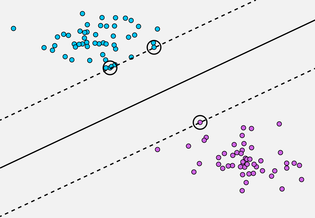
• many lines could separate two clusters of points on a 2D plot, but support vector machine (SVM) finds the best one
• the best line is the one as far as possible from the nearest points in each cluster
  • this line is called the decision boundary
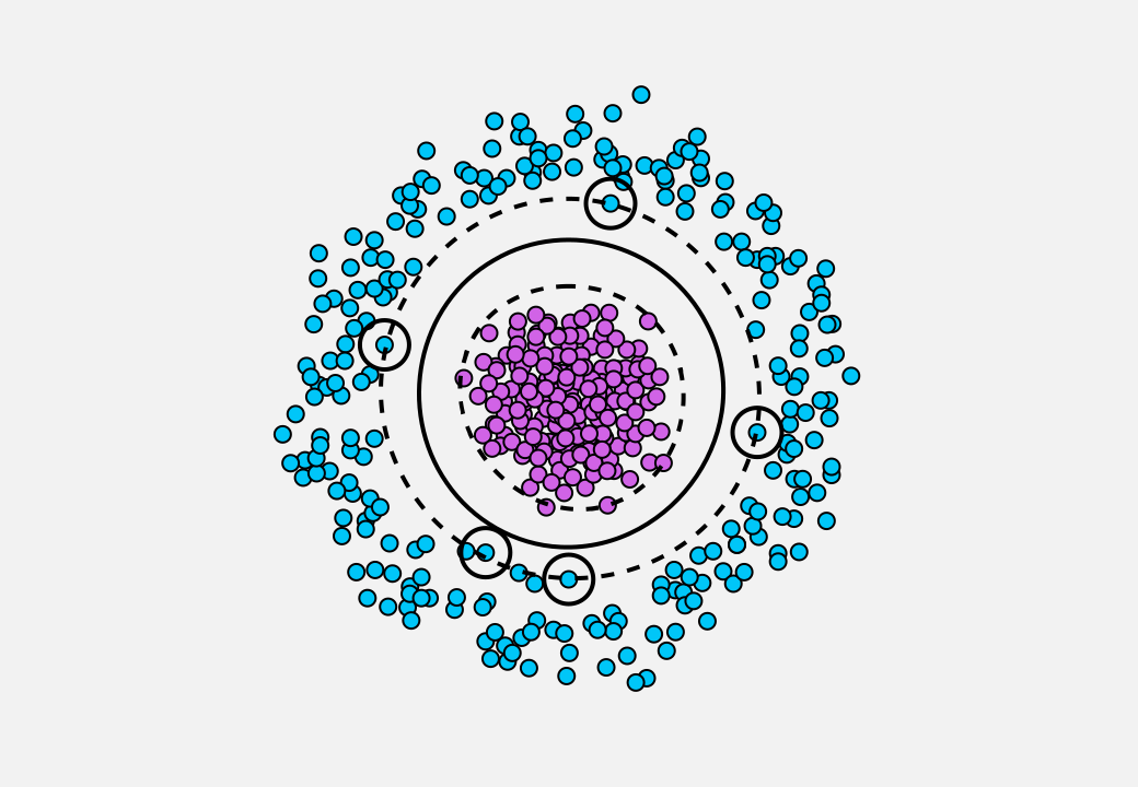
  • circled samples → the nearest samples or the support vectors
  • dashed lines and circles → just visual aids
  • distance from the solid line to the dashed lines → the margin
    • the wider the margin, the better
    • SVM chooses the line with the largest margin

Why support vector machine?

• support = nearest
• vector = data point (sample)
• machine = algorithm
• SVM is basically a "nearest-sample algorithm"

A tunable parameter C controls how strict the SVM is about drawing a clean boundary, allowing it to handle noisy or overlapping data:

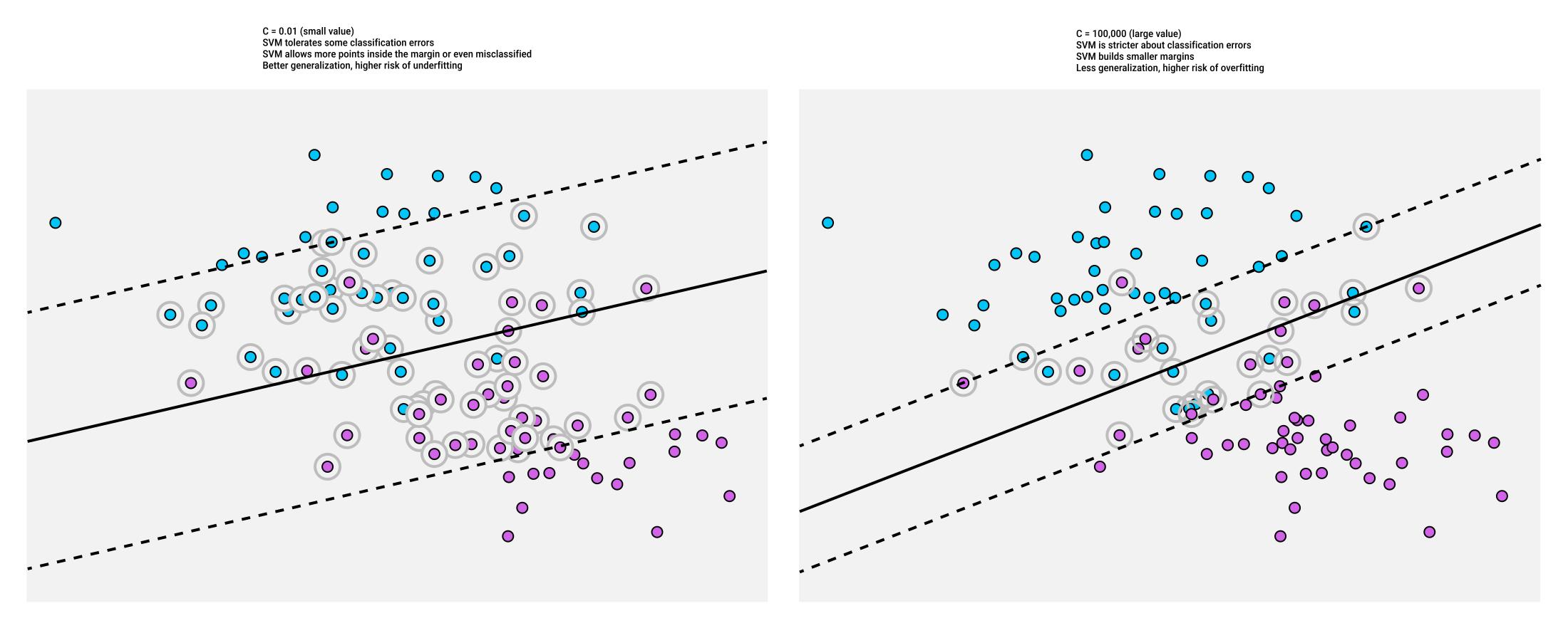
The best value for C is found using trial and error with cross-validation.

The SVM kernel trick

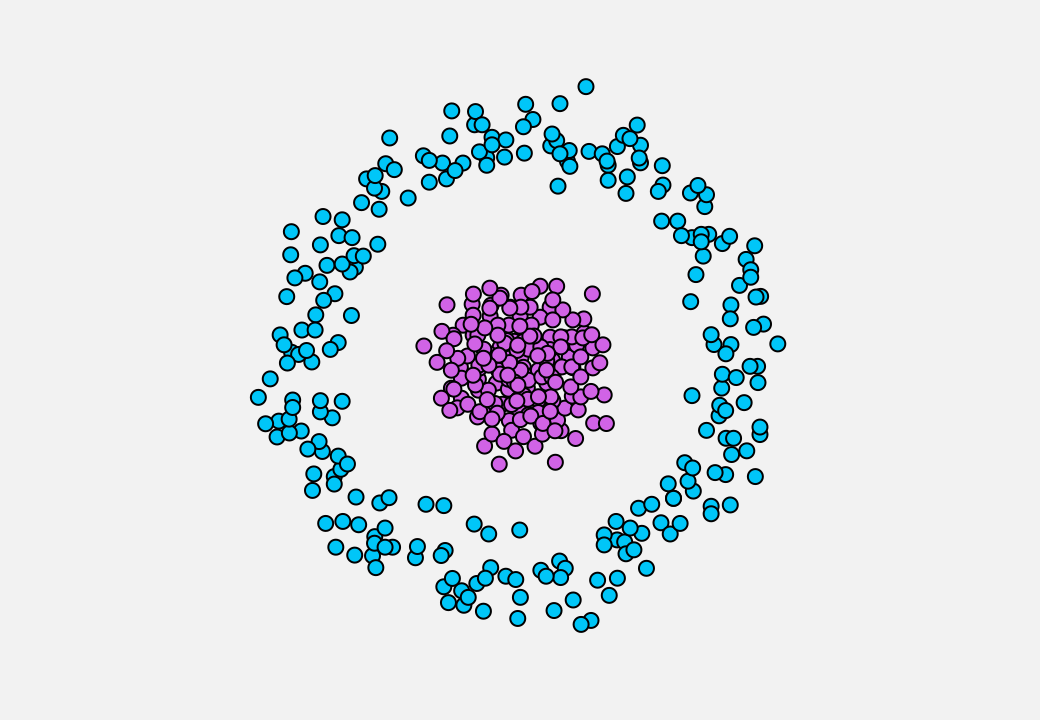
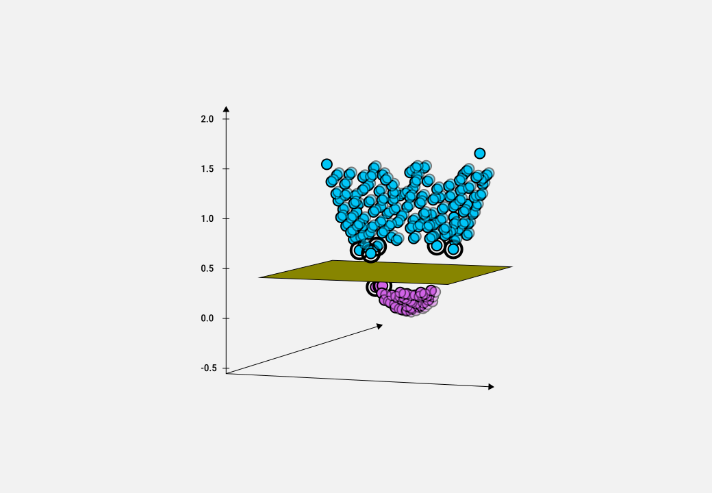
SVMs have limitations when data cannot be separated by a simple linear boundary (e.g., a line or a plane).

The SVM Kernel Trick solves this by transforming data into a higher-dimensional space where a linear separation is possible.

Explanation	Image
One class is surrounded by another, so a straight line cannot separate the two classes.
The trick: add a third dimension to each point elevate each point based on its distance from the center of the pink blob this creates two distinct "clouds" of points, which can be separated by a plane Then the same SVM principles apply for finding the separator (the plane): use support vectors and margins to find the best plane that separates the two classes points above the plane → one class points below the plane → the other This transformation allows the application of the same SVM algorithms but in a higher-dimensional space.
Mapping this back to 2D: circled points = the nearest samples, or the support vectors dashed lines = the margins solid line = the best boundary found by SVM (the separating plane in 3D space)

The kernel trick lets SVM handle high-dimensional data without explicitly transforming it:

• the kernel is a piece of math that lies at the heart of the SVM algorithm
• it's called a "trick" because it cleverly rewrites the SVM math

All major machine learning libraries implement it.

Naive Bayes

Naive Bayes is a parametric classifier based on Bayes' Rule. It gives quick results and often works surprisingly well.

It is called "naive" because it makes strong "naive" assumptions about the data:

• it assumes features are independent (they don't depend on any other one)
• it assumes that features follow a predetermined distribution (often Gaussian) without verifying it

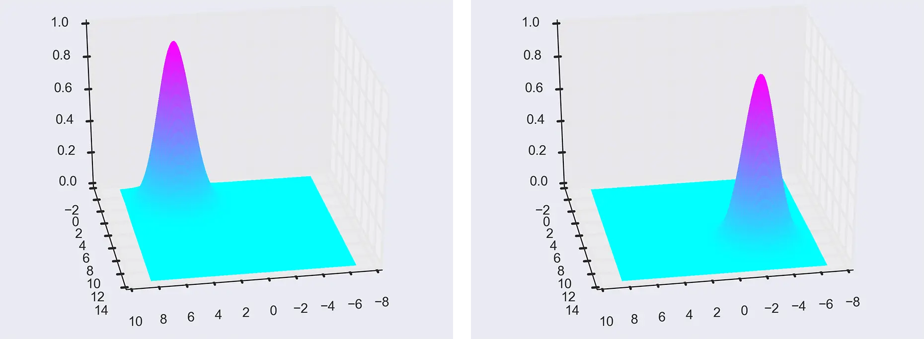
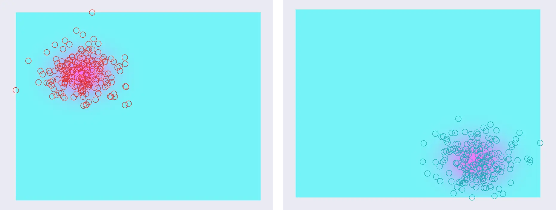
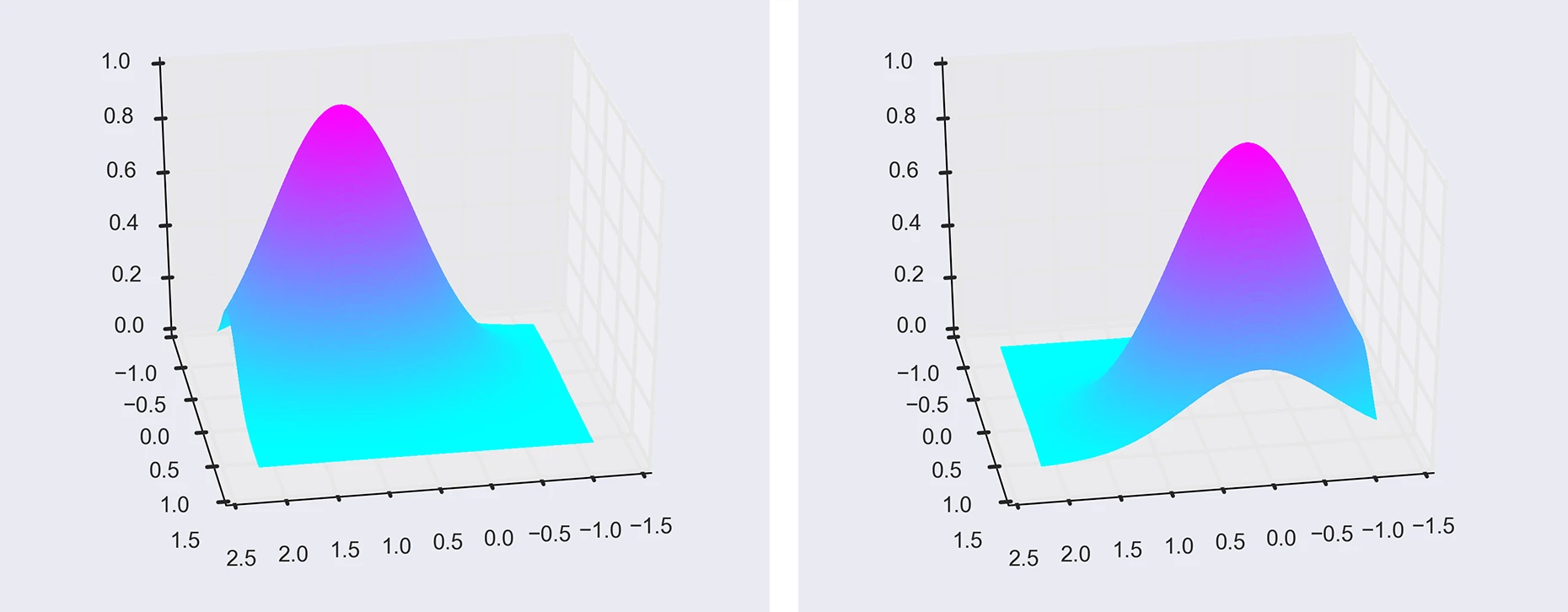
It works by fitting a Gaussian distribution to each feature for each class, then using these fitted distributions to compute class probabilities.

When the data fits the Gaussian assumption (data matches prior):

Explanation	Image
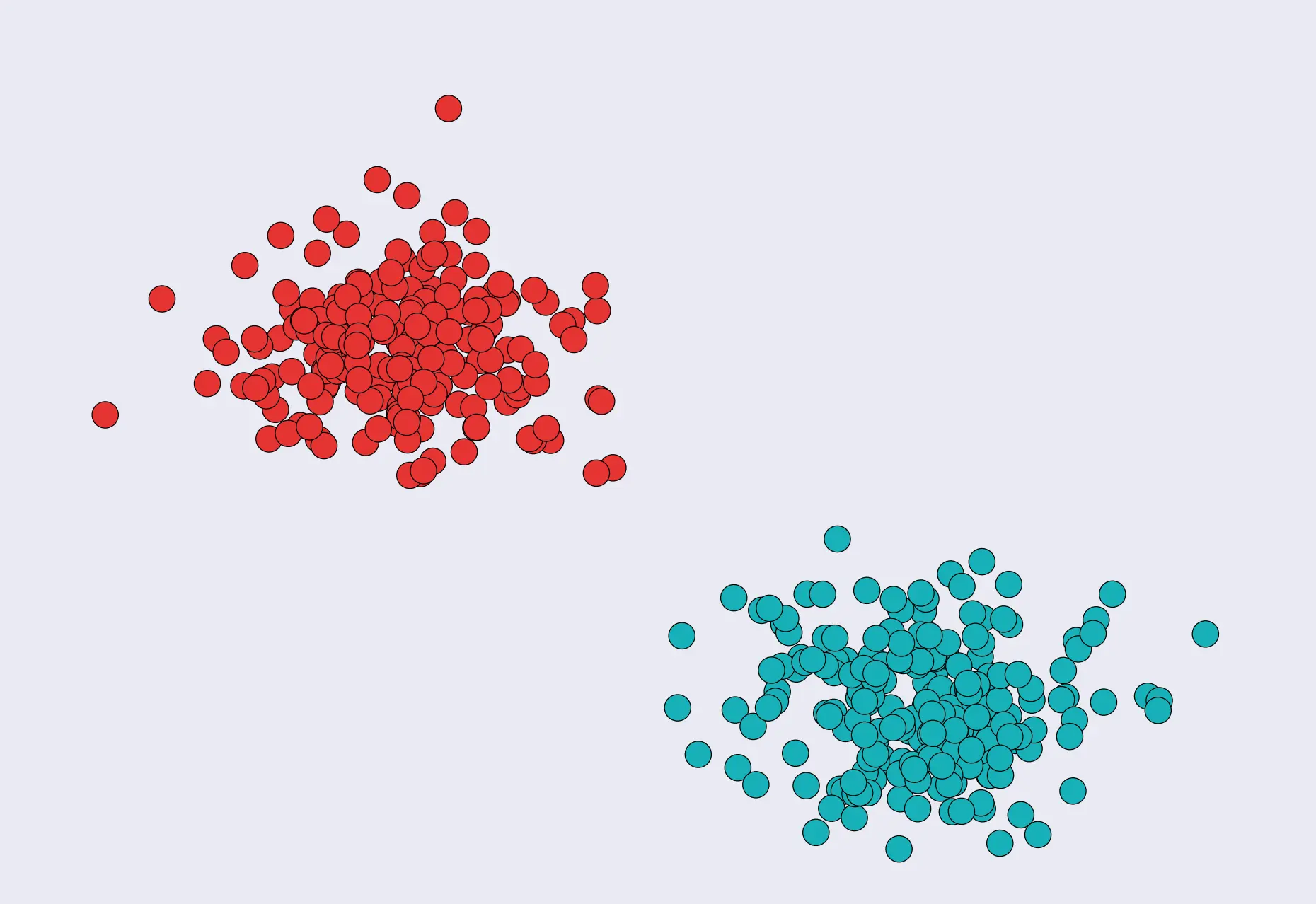
Example: a 2D dataset with red and blue classes.
A Naive Bayes classifier: assumes each feature (x and y) for each class follows a Gaussian tries to fit the best Gaussians to each feature of each class creating two 2D hills
The Gaussian blobs fitted by Naive Bayes closely align with the actual data points. This happens because the model's assumptions match the true underlying data distribution. When the assumptions are correct, the model can separate the classes clearly, resulting in highly accurate classification.

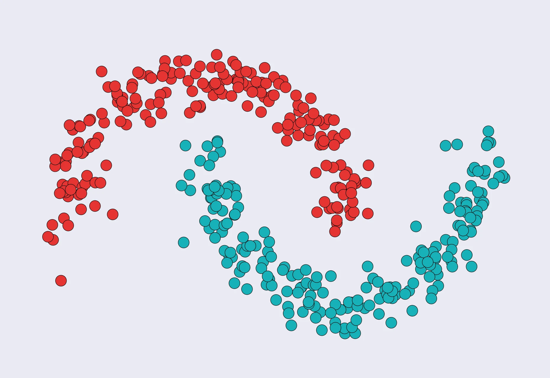
When assumptions fail (data doesn't match prior):

Explanation	Image
If data doesn't follow a Gaussian, like a crescent-shaped cluster, Naive Bayes struggles.
It tries to fit Gaussians anyway.
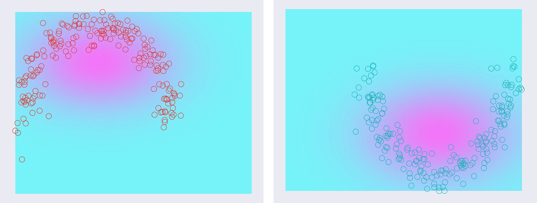
The resulting Gaussian blobs don't match the data well: some points will be misclassified though it may still get many points right

Despite its simplicity, Naive Bayes often performs well, probably because many real-world datasets naturally approximate Gaussian distributions.

Because it relies on simplifying assumptions rather than learning complex relationships, it is computationally efficient and fast.

Comparing classifiers

Algorithm	Pros	Cons
k-Nearest Neighbors	simple to understand and implement very flexible; can model complex class boundaries fast to train (just stores labeled data without performing any calculations)	slow prediction (neighbors must be searched each time) high memory usage (stores all training samples) inefficient for large datasets or real-time systems/websites
Decision Trees	fast to train and make predictions can handle complex decision boundaries easy to interpret and understand	prone to overfitting complex boundaries may require deep trees
Support Vector Machines	fast predictions once trained low memory usage (as it stores only the decision boundaries) kernel trick allows complex decision boundaries	training time increases with the training set size results are sensitive to parameter C (requires tuning, often via cross-validation)
Naive Bayes	very fast training and prediction no hyperparameters needed works well with Gaussian-distributed and high-dimensional datasets reasonably interpretable, because you can look at the Gaussian curves it fits to each feature for each class to see how it makes each prediction	performance can suffer if classes aren't well-separated or if data doesn't follow Gaussian distribution relies on strong (often unrealistic) independence assumptions

These classifiers are commonly used in practice due to their ease of application and visualization:

• especially when exploring new data
• Naive Bayes is often tried first for its speed
• more complex classifiers like SVM or decision trees are considered if needed